── Attaching core tidyverse packages ──────────────────────── tidyverse 2.0.0 ──
✔ dplyr     1.1.4     ✔ readr     2.1.5
✔ forcats   1.0.0     ✔ stringr   1.5.1
✔ ggplot2   3.5.1     ✔ tibble    3.2.1
✔ lubridate 1.9.4     ✔ tidyr     1.3.1
✔ purrr     1.0.4
── Conflicts ────────────────────────────────────────── tidyverse_conflicts() ──
✖ dplyr::filter() masks stats::filter()
✖ dplyr::lag()    masks stats::lag()
ℹ Use the conflicted package (<http://conflicted.r-lib.org/>) to force all conflicts to become errorsR Basics
Loading R packages
In your previous statistics course at Carleton, you likely loaded at least one add-on R package. In this course, we’ll use a lot of tools found in the tidyverse of R packages. To load many of these packages at once, you can use the library(<package_name>) command. So to load the tidyverse we run:
Note
Above we see a lot of extra info printed when we load the tidyverse. These messages are just telling you what packages are now available to you and warning you that a few functions (e.g., filter) has been replaced by the tidyverse version. We’ll see how to suppress these messages later.
Creating and naming objects
All R statements where you create objects have the form:
object_name <- valueAt first, we’ll be creating a lot of data objects. For example, we an load a data set containing the ratings for each episode of The Office using the code
office_ratings <- readr::read_csv("https://raw.githubusercontent.com/rfordatascience/tidytuesday/master/data/2020/2020-03-17/office_ratings.csv")In this class you will be creating a lot of objects, so you’ll need to come up with names for those objects. Trying to think of informative/meaningful names for objects is hard, but necessary work! Below are the fundamental rules for naming objects in R:
- names can’t start with a number
- names are case-sensitive
- some common letters are used internally by R and should be avoided as variable names (
c,q,t,C,D,F,T,I) - There are reserved words that R won’t let you use for variable names (
for,in,while,if,else,repeat,break,next) - R will let you use the name of a predefined function—but don’t do it!
You can always check to see if you the name you want to use is already taken via exists():
For example lm exists
exists("lm")[1] TRUEbut carleton_college doesn’t.
exists("carleton_college")[1] FALSEThere are also a lot of naming styles out there, and if you have coded in another language, you may have already developed a preference. Below is an illustration by Allison Horst
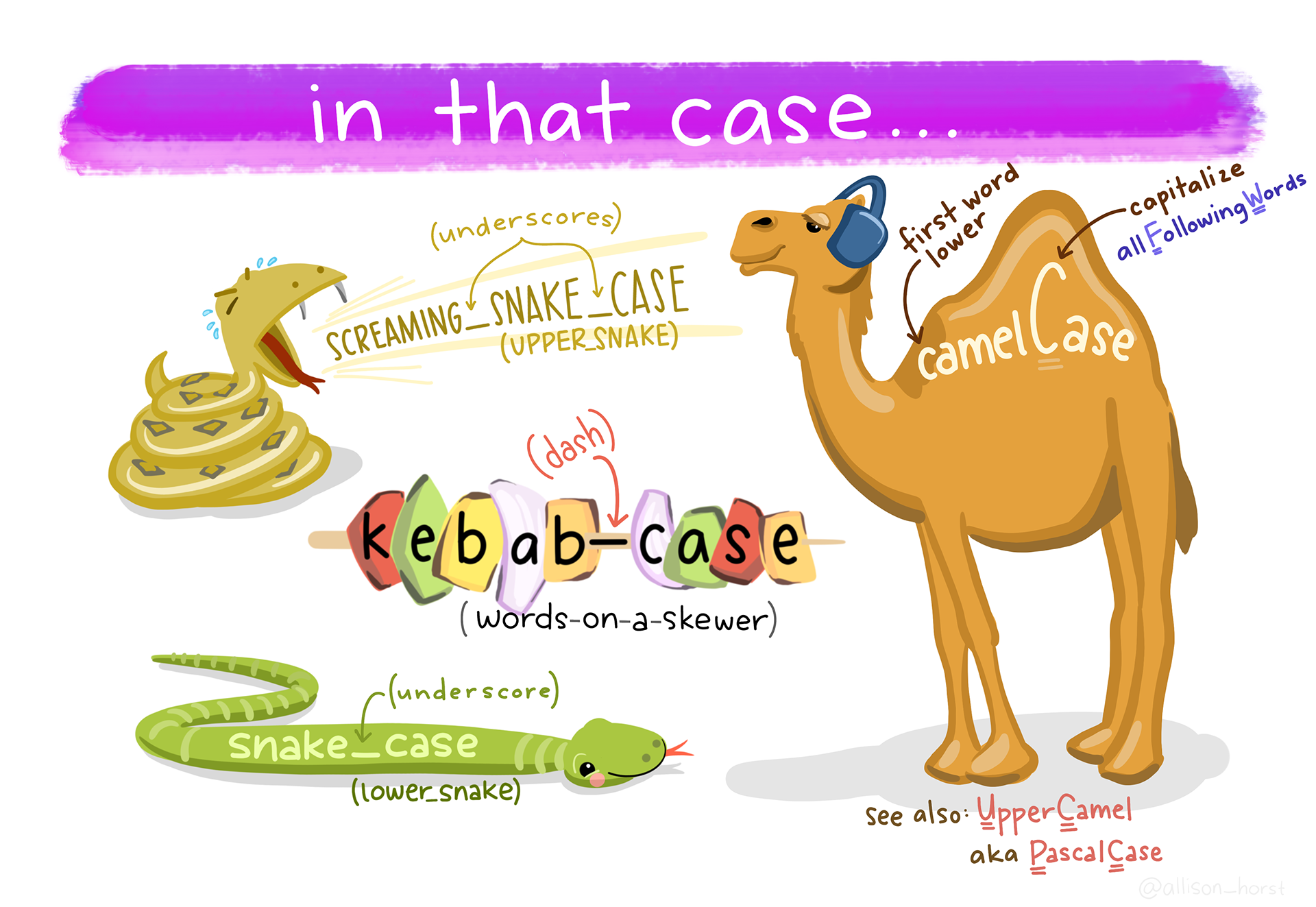
I generally following the tidyverse style guide, so you’ll see that I use only lowercase letters, numbers, and _ (snake case).
Overviews of data frames
Above, you loaded in a data set called office_ratings. Data sets are stored as a special data structure called a data frame. Data frames are the most-commonly used data structure for data analysis in R. For now, think of them like spreadsheets.
Once you have your data frame, you can get a quick overview of it using a few commands (below I use data_set as a generic placeholder for the data frame’s name):
| Command | Description |
|---|---|
head(data_set) |
print the first 6 rows |
tail(data_set) |
print the last 6 rows |
glimpse(data_set) |
a quick overview where columns run down the screen and the data values run across. This allows you to see every column in the data frame. |
str(data_set) |
a quick overview like glimpse(), but without some of the formatting |
summary(data_set) |
quick summary statistics for each column |
dim(data_set) |
the number of rows and columns |
nrow(data_set) |
the number of rows |
ncol(data_set) |
the number of columns |
Tibbles
A tibble, or a tbl_df is another version of a data frame which is used by default in a lot of the tidyverse packages that we’ll use.
Tibbles are data.frames that are lazy and surly: they do less (i.e. they don’t change variable names or types, and don’t do partial matching) and complain more (e.g. when a variable does not exist). This forces you to confront problems earlier, typically leading to cleaner, more expressive code. Tibbles also have an enhanced print() method which makes them easier to use with large datasets containing complex objects.
Getting a spreadsheet
In RStudio, you can run the command View(data_set) to pull up a spreadsheet representation of a data frame. You can also click on the name of the data frame in the Environment pane. This can be a great way help you think about the data, and even has some interactive functions (e.g., filtering and searching); however, never include View(data_set) in an .Rmd file!!
Review from intro stats
In intro stats we used the terms cases (or observations) and variables to describe the rows and columns of a data frame, respectively.
Extracting pieces of data frames
Since data frames are the fundamental data structure for most analyses in R, it’s important to know how to work with them. You already know how to get an overview of a data frame, but that isn’t always very informative. Often, you want to extract pieces of a data frame, such as a specific column or row.
Extracting rows
Data frames can be indexed by their row/column numbers. To extract elements of a data frame, the basic syntax is data_set[row.index, column.index]. So, to extract the 10th row of office_ratings we run
office_ratings[10, ]# A tibble: 1 × 6
season episode title imdb_rating total_votes air_date
<dbl> <dbl> <chr> <dbl> <dbl> <date>
1 2 4 The Fire 8.4 2713 2005-10-11Notice that to extract an entire row, we leave the column index position blank.
We can also extract multiple rows by creating a vector of row indices. For example, we can extract the first 5 rows via
office_ratings[1:5, ]# A tibble: 5 × 6
season episode title imdb_rating total_votes air_date
<dbl> <dbl> <chr> <dbl> <dbl> <date>
1 1 1 Pilot 7.6 3706 2005-03-24
2 1 2 Diversity Day 8.3 3566 2005-03-29
3 1 3 Health Care 7.9 2983 2005-04-05
4 1 4 The Alliance 8.1 2886 2005-04-12
5 1 5 Basketball 8.4 3179 2005-04-19Here, 1:5 create a sequence of integers from 1 to 5.
We could also specify arbitrary row index values by combing the values into a vector. For example, we could extract the 1st, 13th, 64th, and 128th rows via
office_ratings[c(1, 13, 64, 128), ]# A tibble: 4 × 6
season episode title imdb_rating total_votes air_date
<dbl> <dbl> <chr> <dbl> <dbl> <date>
1 1 1 Pilot 7.6 3706 2005-03-24
2 2 7 The Client 8.6 2631 2005-11-08
3 4 13 Job Fair 7.9 1977 2008-05-08
4 7 11 Classy Christmas 8.9 2138 2010-12-09Extracting columns
Similar to extracting rows, we can use a numeric index to extract the columns of a data frame. For example, to extract the 3rd column, we can run
office_ratings[,3]# A tibble: 188 × 1
title
<chr>
1 Pilot
2 Diversity Day
3 Health Care
4 The Alliance
5 Basketball
6 Hot Girl
7 The Dundies
8 Sexual Harassment
9 Office Olympics
10 The Fire
# ℹ 178 more rowsAlternatively, we can pass in the column name in quotes instead of the column number
office_ratings[,"title"]# A tibble: 188 × 1
title
<chr>
1 Pilot
2 Diversity Day
3 Health Care
4 The Alliance
5 Basketball
6 Hot Girl
7 The Dundies
8 Sexual Harassment
9 Office Olympics
10 The Fire
# ℹ 178 more rowsNotice that the extracted column is still formatted as a data frame (or tibble). If you want to extract the contents of the column and just have a vector of titles, you have a few options.
- You could use double brackets with the column number:
office_ratings[[3]]- You could use double brackets with the column name in quotes:
office_ratings[["title"]]- You could use the
$extractor with the column name (not in quotes):
office_ratings$titleLists
It turns out that data frames are special cases of lists, a more general data structure. In a data frame, each column is an element of the data list and each column must be of the same length. In general, lists can be comprised of elements of vastly different lengths and data types.
As an example, let’s construct a list of the faculty in the MAST department and what is being taught this winter.
stat_faculty <- c("Kelling", "Loy", "Luby", "Poppick", "St. Clair", "Wadsworth")
stat_courses <- c(120, 220, 230, 250, 285, 330)
math_faculty <- c("Brooke", "Davis", "Egge", "Gomez-Gonzales", "Haunsperger", "Johnson",
                  "Meyer", "Montee", "Shrestha","Terry", "Thompson", "Turnage-Butterbaugh")
math_courses <- c(101, 106, 111, 120, 210, 211, 232, 236, 240, 241, 251, 321, 333, 395)

mast <- list(stat_faculty = stat_faculty, stat_courses = stat_courses,
             math_faculty = math_faculty, math_courses = math_courses)
Overview of a list
You can get an overview of a list a few ways:
-
glimpse(list_name)andstr(list_name)list the elements of the list and the first few entries of each element.
glimpse(mast)List of 4
$ stat_faculty: chr [1:6] "Kelling" "Loy" "Luby" "Poppick" ...
$ stat_courses: num [1:6] 120 220 230 250 285 330
$ math_faculty: chr [1:12] "Brooke" "Davis" "Egge" "Gomez-Gonzales" ...
$ math_courses: num [1:14] 101 106 111 120 210 211 232 236 240 241 ...-
length(list_name)will tell you how many elements are in the list
length(mast)[1] 4Extracting elements of a list
Since data frames are lists, you’ve already seen how to extract elements of a list. For example, to extract the stat_faculty you could run
mast[[1]][1] "Kelling" "Loy" "Luby" "Poppick" "St. Clair" "Wadsworth"or
mast[["stat_faculty"]][1] "Kelling" "Loy" "Luby" "Poppick" "St. Clair" "Wadsworth"
Note
If you had only used a single bracket above, the returned object would still be a list, which is typically not what we would want.
mast[1]$stat_faculty
[1] "Kelling" "Loy" "Luby" "Poppick" "St. Clair" "Wadsworth"Vectors
The columns of the office_ratings data frame and the elements of the mast list were comprised of (atomic) vectors. Unlike lists, all elements within a vector share the same type. For example, all names in the stat_faculty vector were character strings and all ratings in the imdb_rating column were numeric. We’ll deal with a variety of types of vectors in this course, including:
- numeric
- character (text)
- logical (TRUE/FALSE)
Extracting elements of a vector
Just like with lists (and therefore data frames), we use brackets to extract elements from a vector. As an example, let’s work with the title column from office_ratings.
title <- office_ratings$title # vector of titlesTo extract the 111th title, we run
title[111][1] "New Leads"or two extract the 100th through 111th titles, we run
title[100:111] [1] "Double Date" "Murder" "Shareholder Meeting"
[4] "Scott's Tots" "Secret Santa" "The Banker"
[7] "Sabre" "Manager and Salesman" "The Delivery: Part 1"
[10] "The Delivery: Part 2" "St. Patrick's Day" "New Leads" Negative indices
Sometimes, we want to “kick out” elements of our vector. To do this, we can use a negative index value. For example,
title[-1]returns all but the first title—that is, it kicks out the first title. To kick out multiple elements, we need to negate a vector of indices. For example, below we kick out the first 10 titles
title[-c(1:10)]And now we kick out the 5th, 50th, and 150th titles
title[-c(5, 50, 150)]This idea can be adapted to lists and data frames. For example, to kick out the first row of office_ratings, we run
office_ratings[-1,]# A tibble: 187 × 6
season episode title imdb_rating total_votes air_date
<dbl> <dbl> <chr> <dbl> <dbl> <date>
1 1 2 Diversity Day 8.3 3566 2005-03-29
2 1 3 Health Care 7.9 2983 2005-04-05
3 1 4 The Alliance 8.1 2886 2005-04-12
4 1 5 Basketball 8.4 3179 2005-04-19
5 1 6 Hot Girl 7.8 2852 2005-04-26
6 2 1 The Dundies 8.7 3213 2005-09-20
7 2 2 Sexual Harassment 8.2 2736 2005-09-27
8 2 3 Office Olympics 8.4 2742 2005-10-04
9 2 4 The Fire 8.4 2713 2005-10-11
10 2 5 Halloween 8.2 2561 2005-10-18
# ℹ 177 more rowsor to kick out the math courses from the mast list we run
mast[-4]$stat_faculty
[1] "Kelling" "Loy" "Luby" "Poppick" "St. Clair" "Wadsworth"
$stat_courses
[1] 120 220 230 250 285 330
$math_faculty
[1] "Brooke" "Davis" "Egge"
[4] "Gomez-Gonzales" "Haunsperger" "Johnson"
[7] "Meyer" "Montee" "Shrestha"
[10] "Terry" "Thompson" "Turnage-Butterbaugh"Logical indices
It’s great to be able to extract (or omit) elements using indices, but sometimes we don’t know what index value we should use. For example, if you wanted to extract all of the 300-level statistics courses from the stat_courses vector, you would need to manually determine that positions 2:5 meet that requirement. That’s a lot of work! A better alternative is to allow R to find the elements meeting that requirement using logical operators. Below is a table summarizing common logical operators in R.
| Comparison | Meaning |
|---|---|
< |
less than |
> |
greater than |
<= |
less than or equal to |
>= |
greater than or equal to |
== |
is equal to |
!= |
not equal to |
In order to extract the 300-level statistics courses, we’ll take two steps:
- We’ll determine whether each course is numbered at least 300,
- then we’ll use that sequence of TRUEs/FALSEs to extract the course.
So, first we use the logical operator >= to compare stat_courses and 300. This returns TRUE if the element meets the specification and FALSE otherwise.
stat_courses >= 300[1] FALSE FALSE FALSE FALSE FALSE TRUENow, we can use this vector as our index. Only the TRUE elements will be extracted:
stat_courses[stat_courses >= 300][1] 330The same idea can be used with data frames and lists, just remember how to format the brackets and indices!