Data Wrangling:
Verbs

Day 07

Prof Amanda Luby

Carleton College
Stat 220 - Spring 2025

{dplyr}

A package that transforms data
Implements a grammar of transforming tabular data
Part of the tidyverse

Warm up

With your neighbors, identify the data verb (function) that does the following:

Picks rows by their values
Reorders the rows
Picks variables by their names
Creates new variables with functions of existing variables

02:30

Logical tests

For help:

?Comparison

Syntax	Description
`x < y`	less than
`x > y`	greater than
`x <= y`	less than or equal to
`x >= y`	greater than or equal to
`x == y`	equal to
`x != y`	not equal to
`x %in% y`	group membership
`is.na(x)`	is NA (missing)
`!is.na(x)`	is not NA

Your turn:

With your neighbors, use filter() to wrangle the nycflights23::flights data frame.

Find all flights that had an arrival delay of two or more hours.
Find all flights to MSP
Find all flights that arrived more than two hours late, but left less than one hour late
(if time) Find all flights that were delayed by at least an hour, but made up over 30 minutes in flight.

05:00

`slice(.data, ...)`

Extract (omit) rows by row number

Slicing flights data

Extracting rows 10 to 20

slice(flights, 10:20)

# A tibble: 11 × 19
    year month   day dep_time sched_dep_time dep_delay arr_time sched_arr_time
   <int> <int> <int>    <int>          <int>     <dbl>    <int>          <int>
 1  2023     1     1      547            545         2      845            852
 2  2023     1     1      549            559       -10      905            901
 3  2023     1     1      551            600        -9      846            859
 4  2023     1     1      552            559        -7      857            911
 5  2023     1     1      554            600        -6      914            920
 6  2023     1     1      554            600        -6      725            735
 7  2023     1     1      558            605        -7      719            750
 8  2023     1     1      600            600         0      729            752
 9  2023     1     1      600            600         0      745            755
10  2023     1     1      600            600         0      810            840
11  2023     1     1      603            605        -2      800            818
# ℹ 11 more variables: arr_delay <dbl>, carrier <chr>, flight <int>,
#   tailnum <chr>, origin <chr>, dest <chr>, air_time <dbl>, distance <dbl>,
#   hour <dbl>, minute <dbl>, time_hour <dttm>

Slicing flights data

Omitting rows 100 to 1000

slice(flights, -c(100:1000))

# A tibble: 434,451 × 19
    year month   day dep_time sched_dep_time dep_delay arr_time sched_arr_time
   <int> <int> <int>    <int>          <int>     <dbl>    <int>          <int>
 1  2023     1     1        1           2038       203      328              3
 2  2023     1     1       18           2300        78      228            135
 3  2023     1     1       31           2344        47      500            426
 4  2023     1     1       33           2140       173      238           2352
 5  2023     1     1       36           2048       228      223           2252
 6  2023     1     1      503            500         3      808            815
 7  2023     1     1      520            510        10      948            949
 8  2023     1     1      524            530        -6      645            710
 9  2023     1     1      537            520        17      926            818
10  2023     1     1      547            545         2      845            852
# ℹ 434,441 more rows
# ℹ 11 more variables: arr_delay <dbl>, carrier <chr>, flight <int>,
#   tailnum <chr>, origin <chr>, dest <chr>, air_time <dbl>, distance <dbl>,
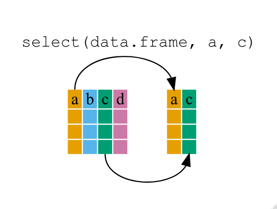
#   hour <dbl>, minute <dbl>, time_hour <dttm>

`select()`

Extract columns by name or number

select(.data, ...)

Storms data

glimpse(storms)

Rows: 19,537
Columns: 13
$ name                         <chr> "Amy", "Amy", "Amy", "Amy", "Amy", "Amy",…
$ year                         <dbl> 1975, 1975, 1975, 1975, 1975, 1975, 1975,…
$ month                        <dbl> 6, 6, 6, 6, 6, 6, 6, 6, 6, 6, 6, 6, 6, 6,…
$ day                          <int> 27, 27, 27, 27, 28, 28, 28, 28, 29, 29, 2…
$ hour                         <dbl> 0, 6, 12, 18, 0, 6, 12, 18, 0, 6, 12, 18,…
$ lat                          <dbl> 27.5, 28.5, 29.5, 30.5, 31.5, 32.4, 33.3,…
$ long                         <dbl> -79.0, -79.0, -79.0, -79.0, -78.8, -78.7,…
$ status                       <fct> tropical depression, tropical depression,…
$ category                     <dbl> NA, NA, NA, NA, NA, NA, NA, NA, NA, NA, N…
$ wind                         <int> 25, 25, 25, 25, 25, 25, 25, 30, 35, 40, 4…
$ pressure                     <int> 1013, 1013, 1013, 1013, 1012, 1012, 1011,…
$ tropicalstorm_force_diameter <int> NA, NA, NA, NA, NA, NA, NA, NA, NA, NA, N…
$ hurricane_force_diameter     <int> NA, NA, NA, NA, NA, NA, NA, NA, NA, NA, N…

select range of columns

select(storms, status:pressure)

# A tibble: 19,537 × 4
   status              category  wind pressure
   <fct>                  <dbl> <int>    <int>
 1 tropical depression       NA    25     1013
 2 tropical depression       NA    25     1013
 3 tropical depression       NA    25     1013
 4 tropical depression       NA    25     1013
 5 tropical depression       NA    25     1012
 6 tropical depression       NA    25     1012
 7 tropical depression       NA    25     1011
 8 tropical depression       NA    30     1006
 9 tropical storm            NA    35     1004
10 tropical storm            NA    40     1002
# ℹ 19,527 more rows

select every column but

select(storms, -c(status, pressure))

# A tibble: 19,537 × 11
   name   year month   day  hour   lat  long category  wind
   <chr> <dbl> <dbl> <int> <dbl> <dbl> <dbl>    <dbl> <int>
 1 Amy    1975     6    27     0  27.5 -79         NA    25
 2 Amy    1975     6    27     6  28.5 -79         NA    25
 3 Amy    1975     6    27    12  29.5 -79         NA    25
 4 Amy    1975     6    27    18  30.5 -79         NA    25
 5 Amy    1975     6    28     0  31.5 -78.8       NA    25
 6 Amy    1975     6    28     6  32.4 -78.7       NA    25
 7 Amy    1975     6    28    12  33.3 -78         NA    25
 8 Amy    1975     6    28    18  34   -77         NA    30
 9 Amy    1975     6    29     0  34.4 -75.8       NA    35
10 Amy    1975     6    29     6  34   -74.8       NA    40
# ℹ 19,527 more rows
# ℹ 2 more variables: tropicalstorm_force_diameter <int>,
#   hurricane_force_diameter <int>

select columns that start with…

select(storms, starts_with("w"))

# A tibble: 19,537 × 1
    wind
   <int>
 1    25
 2    25
 3    25
 4    25
 5    25
 6    25
 7    25
 8    30
 9    35
10    40
# ℹ 19,527 more rows

select columns that end with…

select(storms, ends_with("e"))

# A tibble: 19,537 × 2
   name  pressure
   <chr>    <int>
 1 Amy       1013
 2 Amy       1013
 3 Amy       1013
 4 Amy       1013
 5 Amy       1012
 6 Amy       1012
 7 Amy       1011
 8 Amy       1006
 9 Amy       1004
10 Amy       1002
# ℹ 19,527 more rows

select columns whose names contain…

select(storms, contains("d"))

# A tibble: 19,537 × 4
     day  wind tropicalstorm_force_diameter hurricane_force_diameter
   <int> <int>                        <int>                    <int>
 1    27    25                           NA                       NA
 2    27    25                           NA                       NA
 3    27    25                           NA                       NA
 4    27    25                           NA                       NA
 5    28    25                           NA                       NA
 6    28    25                           NA                       NA
 7    28    25                           NA                       NA
 8    28    30                           NA                       NA
 9    29    35                           NA                       NA
10    29    40                           NA                       NA
# ℹ 19,527 more rows

Try it:

Brainstorm as many ways as possible to select() the following columns from flight:

dep_time
dep_delay
arr_time
arr_delay

02:00

`arrange()`

Order rows from smallest to largest

Arranging by wind speed

By default, arrange orders in ascending order

Original Data
Ascending
Descending

storms

# A tibble: 19,537 × 13
   name   year month   day  hour   lat  long status      category  wind pressure
   <chr> <dbl> <dbl> <int> <dbl> <dbl> <dbl> <fct>          <dbl> <int>    <int>
 1 Amy    1975     6    27     0  27.5 -79   tropical d…       NA    25     1013
 2 Amy    1975     6    27     6  28.5 -79   tropical d…       NA    25     1013
 3 Amy    1975     6    27    12  29.5 -79   tropical d…       NA    25     1013
 4 Amy    1975     6    27    18  30.5 -79   tropical d…       NA    25     1013
 5 Amy    1975     6    28     0  31.5 -78.8 tropical d…       NA    25     1012
 6 Amy    1975     6    28     6  32.4 -78.7 tropical d…       NA    25     1012
 7 Amy    1975     6    28    12  33.3 -78   tropical d…       NA    25     1011
 8 Amy    1975     6    28    18  34   -77   tropical d…       NA    30     1006
 9 Amy    1975     6    29     0  34.4 -75.8 tropical s…       NA    35     1004
10 Amy    1975     6    29     6  34   -74.8 tropical s…       NA    40     1002
# ℹ 19,527 more rows
# ℹ 2 more variables: tropicalstorm_force_diameter <int>,
#   hurricane_force_diameter <int>

arrange(storms, wind)

# A tibble: 19,537 × 13
   name      year month   day  hour   lat  long status   category  wind pressure
   <chr>    <dbl> <dbl> <int> <dbl> <dbl> <dbl> <fct>       <dbl> <int>    <int>
 1 Bonnie    1986     6    28     6  36.5 -91.3 tropica…       NA    10     1013
 2 Bonnie    1986     6    28    12  37.2 -90   tropica…       NA    10     1012
 3 Charley   1986     8    13    12  30.1 -84   subtrop…       NA    10     1009
 4 Charley   1986     8    13    18  30.8 -84   subtrop…       NA    10     1012
 5 Charley   1986     8    14     0  31.4 -83.6 subtrop…       NA    10     1013
 6 Charley   1986     8    14     6  32   -83.1 subtrop…       NA    10     1014
 7 Charley   1986     8    14    12  32.5 -82.5 subtrop…       NA    10     1015
 8 Charley   1986     8    14    18  32.4 -82   subtrop…       NA    10     1015
 9 AL031987  1987     8    16    18  30.9 -83.2 tropica…       NA    10     1014
10 AL031987  1987     8    17     0  31.4 -82.9 tropica…       NA    10     1015
# ℹ 19,527 more rows
# ℹ 2 more variables: tropicalstorm_force_diameter <int>,
#   hurricane_force_diameter <int>

arrange(storms, desc(wind))

# A tibble: 19,537 × 13
   name     year month   day  hour   lat  long status    category  wind pressure
   <chr>   <dbl> <dbl> <int> <dbl> <dbl> <dbl> <fct>        <dbl> <int>    <int>
 1 Allen    1980     8     7    18  21.8 -86.4 hurricane        5   165      899
 2 Gilbert  1988     9    14     0  19.7 -83.8 hurricane        5   160      888
 3 Wilma    2005    10    19    12  17.3 -82.8 hurricane        5   160      882
 4 Dorian   2019     9     1    16  26.5 -77   hurricane        5   160      910
 5 Dorian   2019     9     1    18  26.5 -77.1 hurricane        5   160      910
 6 Allen    1980     8     5    12  15.9 -70.5 hurricane        5   155      932
 7 Allen    1980     8     7    12  21   -84.8 hurricane        5   155      910
 8 Allen    1980     8     8     0  22.2 -87.9 hurricane        5   155      920
 9 Allen    1980     8     9     6  25   -94.2 hurricane        5   155      909
10 Gilbert  1988     9    14     6  19.9 -85.3 hurricane        5   155      889
# ℹ 19,527 more rows
# ℹ 2 more variables: tropicalstorm_force_diameter <int>,
#   hurricane_force_diameter <int>

Try it:

Use arrange to answer the following questions:

Which flights traveled the farthest?
Which traveled the shortest?
Which flights lasted the longest?
Which lasted the shortest?

02:30

`slice_min(.data, order_by, n)`

select rows with n smallest values of a variable

`slice_max(.data, order_by, n)`

select rows with n largest values of a variable

Continuing storms example

slice_max
slice_min

Extracting storms with 3 highest wind speeds

slice_max(storms, wind, n = 3)

# A tibble: 5 × 13
  name     year month   day  hour   lat  long status    category  wind pressure
  <chr>   <dbl> <dbl> <int> <dbl> <dbl> <dbl> <fct>        <dbl> <int>    <int>
1 Allen    1980     8     7    18  21.8 -86.4 hurricane        5   165      899
2 Gilbert  1988     9    14     0  19.7 -83.8 hurricane        5   160      888
3 Wilma    2005    10    19    12  17.3 -82.8 hurricane        5   160      882
4 Dorian   2019     9     1    16  26.5 -77   hurricane        5   160      910
5 Dorian   2019     9     1    18  26.5 -77.1 hurricane        5   160      910
# ℹ 2 more variables: tropicalstorm_force_diameter <int>,
#   hurricane_force_diameter <int>

Extracting storms with the lowest wind speed

slice_min(storms, wind, n = 1)

# A tibble: 61 × 13
   name      year month   day  hour   lat  long status   category  wind pressure
   <chr>    <dbl> <dbl> <int> <dbl> <dbl> <dbl> <fct>       <dbl> <int>    <int>
 1 Bonnie    1986     6    28     6  36.5 -91.3 tropica…       NA    10     1013
 2 Bonnie    1986     6    28    12  37.2 -90   tropica…       NA    10     1012
 3 Charley   1986     8    13    12  30.1 -84   subtrop…       NA    10     1009
 4 Charley   1986     8    13    18  30.8 -84   subtrop…       NA    10     1012
 5 Charley   1986     8    14     0  31.4 -83.6 subtrop…       NA    10     1013
 6 Charley   1986     8    14     6  32   -83.1 subtrop…       NA    10     1014
 7 Charley   1986     8    14    12  32.5 -82.5 subtrop…       NA    10     1015
 8 Charley   1986     8    14    18  32.4 -82   subtrop…       NA    10     1015
 9 AL031987  1987     8    16    18  30.9 -83.2 tropica…       NA    10     1014
10 AL031987  1987     8    17     0  31.4 -82.9 tropica…       NA    10     1015
# ℹ 51 more rows
# ℹ 2 more variables: tropicalstorm_force_diameter <int>,
#   hurricane_force_diameter <int>

Star Wars character BMI

{dplyr} includes a starwars data frame with characteristics of 87 Star Wars characters

glimpse(starwars)

Rows: 87
Columns: 14
$ name       <chr> "Luke Skywalker", "C-3PO", "R2-D2", "Darth Vader", "Leia Or…
$ height     <int> 172, 167, 96, 202, 150, 178, 165, 97, 183, 182, 188, 180, 2…
$ mass       <dbl> 77.0, 75.0, 32.0, 136.0, 49.0, 120.0, 75.0, 32.0, 84.0, 77.…
$ hair_color <chr> "blond", NA, NA, "none", "brown", "brown, grey", "brown", N…
$ skin_color <chr> "fair", "gold", "white, blue", "white", "light", "light", "…
$ eye_color  <chr> "blue", "yellow", "red", "yellow", "brown", "blue", "blue",…
$ birth_year <dbl> 19.0, 112.0, 33.0, 41.9, 19.0, 52.0, 47.0, NA, 24.0, 57.0, …
$ sex        <chr> "male", "none", "none", "male", "female", "male", "female",…
$ gender     <chr> "masculine", "masculine", "masculine", "masculine", "femini…
$ homeworld  <chr> "Tatooine", "Tatooine", "Naboo", "Tatooine", "Alderaan", "T…
$ species    <chr> "Human", "Droid", "Droid", "Human", "Human", "Human", "Huma…
$ films      <list> <"A New Hope", "The Empire Strikes Back", "Return of the J…
$ vehicles   <list> <"Snowspeeder", "Imperial Speeder Bike">, <>, <>, <>, "Imp…
$ starships  <list> <"X-wing", "Imperial shuttle">, <>, <>, "TIE Advanced x1",…

Star Wars character BMI

Suppose we want to calculate the BMI for each character, \(\text{BMI} = \dfrac{\text{mass (kg)}}{\text{height (m)}^2}\)

starwars <- mutate(starwars, bmi = mass / (height / 100)^2)

select(starwars, name, bmi, everything())

# A tibble: 87 × 15
   name        bmi height  mass hair_color skin_color eye_color birth_year sex  
   <chr>     <dbl>  <int> <dbl> <chr>      <chr>      <chr>          <dbl> <chr>
 1 Luke Sky…  26.0    172    77 blond      fair       blue            19   male 
 2 C-3PO      26.9    167    75 <NA>       gold       yellow         112   none 
 3 R2-D2      34.7     96    32 <NA>       white, bl… red             33   none 
 4 Darth Va…  33.3    202   136 none       white      yellow          41.9 male 
 5 Leia Org…  21.8    150    49 brown      light      brown           19   fema…
 6 Owen Lars  37.9    178   120 brown, gr… light      blue            52   male 
 7 Beru Whi…  27.5    165    75 brown      light      blue            47   fema…
 8 R5-D4      34.0     97    32 <NA>       white, red red             NA   none 
 9 Biggs Da…  25.1    183    84 black      light      brown           24   male 
10 Obi-Wan …  23.2    182    77 auburn, w… fair       blue-gray       57   male 
# ℹ 77 more rows
# ℹ 6 more variables: gender <chr>, homeworld <chr>, species <chr>,
#   films <list>, vehicles <list>, starships <list>

Try it

Create a new column in flights giving the average speed of the flight while it was in the air. What are the units of this variable? Make the variable in terms of miles per hour.

02:30

Example

The Federal Aviation Administration (FAA) considers a flight to be delayed when it is 15 minutes later than its scheduled time.

flights <- mutate(
  flights, 
  delayed = case_when(
    dep_delay >= 15 ~ "Delayed", 
    dep_delay < 15 ~ "On time",
    .default = "other")
)

Your turn

Suppose that you don’t think the FAA gives enough information in their definition of a delayed flight, so you come up with the following delay categories:

dep_delay <= 0 -> none
dep_delay between 1 and 15 minutes -> minimal
dep_delay between 16 and 30 minutes -> delayed
dep_delay between 31 and 60 minutes -> major
dep_delay over 60 minutes -> extreme

Use mutate() and case_when() to create a delay_category variable in the flights data frame.

`%>% or |>`

“dataframe first, dataframe once”
Combine multiple operations with the pipe
Think “and then” when reading code

Using `%>%` or `|>`

%>% or |> passes result on left into first argument of function on right
Chaining functions together lets you read Left-to-right, top-to-bottom

Using `%>% or |>`

`filter()`:

filter(storms, status == "hurricane")

becomes

storms %>%
  filter(status == "hurricane")

`arrange()`:

arrange(storms, wind)

becomes

storms |>
  arrange(wind)

Using `%>%` or `|>`

We can also build up a series of pipes.

We’re interested in the storms with the lowest wind speed that were still classified as hurricanes.

storms %>%
  filter(status == "hurricane") %>%
  arrange(wind)

# A tibble: 4,803 × 13
   name      year month   day  hour   lat  long status   category  wind pressure
   <chr>    <dbl> <dbl> <int> <dbl> <dbl> <dbl> <fct>       <dbl> <int>    <int>
 1 Blanche   1975     7    27     6  35.9 -70   hurrica…        1    65      987
 2 Caroline  1975     8    30     0  23.3 -94.2 hurrica…        1    65      990
 3 Caroline  1975     8    30     6  23.5 -94.9 hurrica…        1    65      990
 4 Caroline  1975     8    30    12  23.7 -95.6 hurrica…        1    65      989
 5 Doris     1975     8    31     0  34.9 -46.3 hurrica…        1    65      990
 6 Doris     1975     8    31     6  34.8 -45.7 hurrica…        1    65      990
 7 Eloise    1975     9    16    18  19.5 -68.4 hurrica…        1    65     1002
 8 Eloise    1975     9    17     0  19.6 -69.2 hurrica…        1    65      997
 9 Eloise    1975     9    22     6  24.8 -89.4 hurrica…        1    65      993
10 Faye      1975     9    26     0  26.5 -60   hurrica…        1    65      990
# ℹ 4,793 more rows
# ℹ 2 more variables: tropicalstorm_force_diameter <int>,
#   hurricane_force_diameter <int>

Using `%>%` or `|>`

We’re interested in the storms with the lowest wind speed that were still classified as hurricanes, that reached category 2.

storms %>%
  filter(status == "hurricane") %>%
  filter(category > 1) %>%
  arrange(wind)

# A tibble: 2,255 × 13
   name    year month   day  hour   lat  long status    category  wind pressure
   <chr>  <dbl> <dbl> <int> <dbl> <dbl> <dbl> <fct>        <dbl> <int>    <int>
 1 Eloise  1975     9    22    18  26.5 -89.4 hurricane        2    85      980
 2 Faye    1975     9    26    18  31   -63.1 hurricane        2    85      985
 3 Faye    1975     9    28     0  38.4 -63.7 hurricane        2    85      985
 4 Gladys  1975    10     3     6  43.7 -57   hurricane        2    85      960
 5 Gladys  1975    10     3    12  46.6 -50.6 hurricane        2    85      960
 6 Emmy    1976     8    26    18  27.7 -54.8 hurricane        2    85      976
 7 Emmy    1976     8    27    12  30.9 -53.7 hurricane        2    85      975
 8 Emmy    1976     8    28    12  33.5 -56.6 hurricane        2    85      975
 9 Emmy    1976     8    31    12  35.1 -44.9 hurricane        2    85      977
10 Gloria  1976     9    30     6  32.2 -59.8 hurricane        2    85      971
# ℹ 2,245 more rows
# ℹ 2 more variables: tropicalstorm_force_diameter <int>,
#   hurricane_force_diameter <int>

Combining with `ggplot`

Pipes become especially useful when we combine them with ggplot():

storms |>
  filter(status == "hurricane") |>
  filter(category > 1) |>
  ggplot(aes(x = wind, y = hurricane_force_diameter)) + 
  geom_jitter() +
  labs(
    title = "Force diameter vs wind speed",
    subtitle = "Hurricanes only"
  )

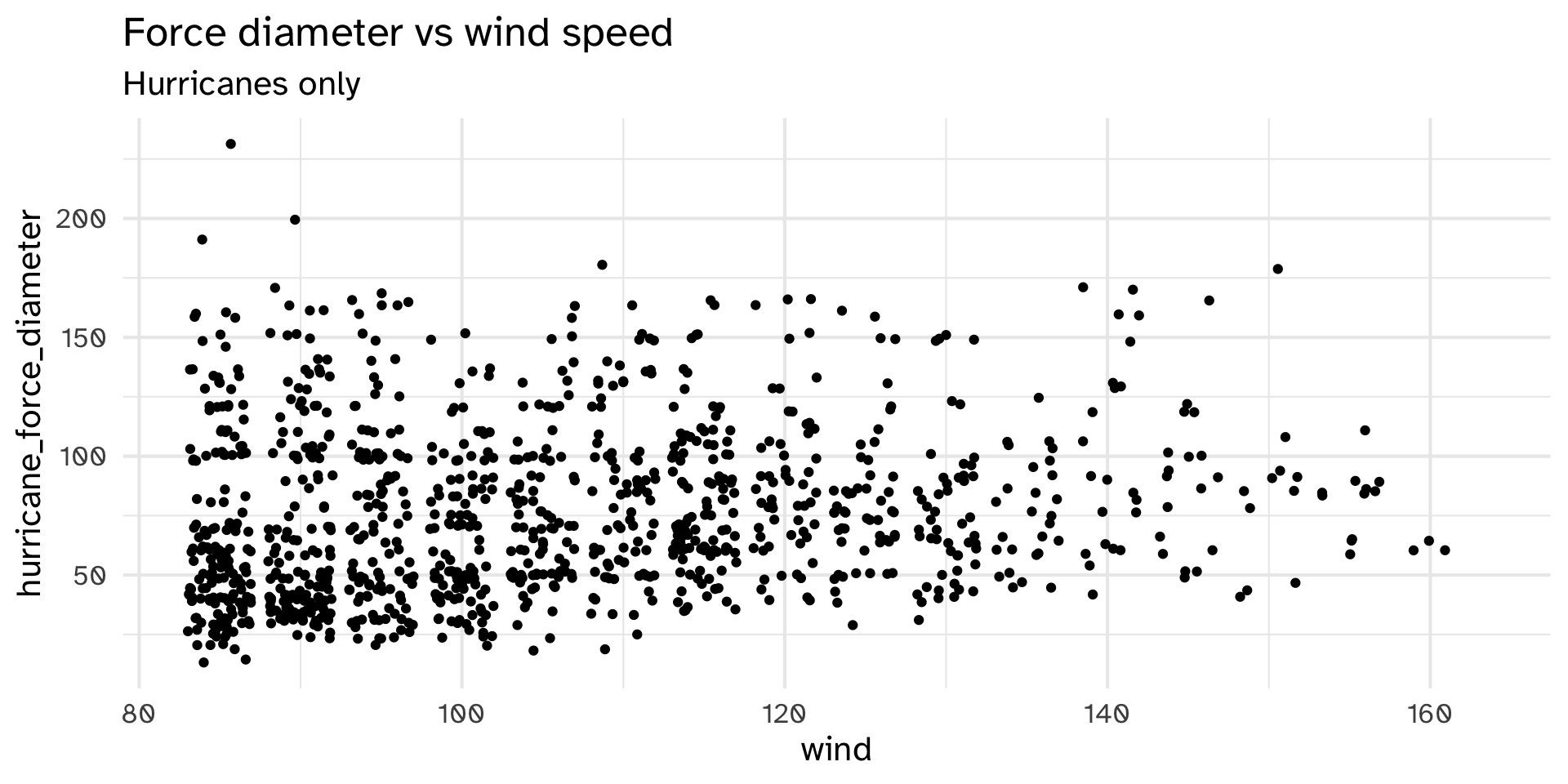
Your turn

Chain the last two parts together, so that the resulting dataset contains both avg_speed and delay_category. Pipe this new dataset into ggplot() to answer the question “is there a relationship between average speed and how late a flight is delayed?”

If you have time, create a new graph which only contains flights to MSP.

04:00

Data Wrangling: Verbs

{dplyr}

Warm up

Logical tests

Your turn:

slice(.data, ...)

Slicing flights data

Slicing flights data

select()

Storms data

select() helpers

Try it:

arrange()

Arranging by wind speed

Try it:

slice_min(.data, order_by, n)

slice_max(.data, order_by, n)

Continuing storms example

Star Wars character BMI

Star Wars character BMI

Try it

Example

Your turn

%>% or |>

Using %>% or |>

Using %>% or |>

filter():

arrange():

Using %>% or |>

Using %>% or |>

Combining with ggplot

Your turn

Lab Quiz 1

Data Wrangling:
Verbs

`slice(.data, ...)`

`select()`

`select()` helpers

`arrange()`

`slice_min(.data, order_by, n)`

`slice_max(.data, order_by, n)`

`%>% or |>`

Using `%>%` or `|>`

Using `%>% or |>`

`filter()`:

`arrange()`:

Using `%>%` or `|>`

Using `%>%` or `|>`

Combining with `ggplot`