Data Wrangling:
Groups &
Tidy Data

Day 08

Prof Amanda Luby

Carleton College
Stat 220 - Spring 2025

The College Scorecard

The College Scorecard is designed to increase transparency, putting the power in the hands of the public — from those choosing colleges to those improving college quality — to see how well different schools are serving their students.

Rows: 187
Columns: 13
$ unitid         <dbl> 228343, 177719, 367884, 149781, 135364, 212601, 133979,…
$ school         <chr> "Southwestern University", "Barnes-Jewish College Goldf…
$ type           <chr> "private", "private", "private", "private", "private", …
$ city           <chr> "Georgetown", "Saint Louis", "Fort Myers", "Wheaton", "…
$ state          <chr> "TX", "MO", "FL", "IL", "GA", "PA", "FL", "CA", "IN", "…
$ region         <chr> "Southwest", "Plains", "Southeast", "Great Lakes", "Sou…
$ admission_rate <dbl> 0.4903, NA, 0.6121, 0.8481, 0.5000, 0.7552, 0.3999, 0.5…
$ act            <dbl> 26, NA, NA, 29, NA, 23, NA, 22, 25, 31, NA, NA, 20, 20,…
$ undergrads     <dbl> 1507, 569, 832, 2358, 235, 2866, 1049, 4516, 2120, 1545…
$ cost           <dbl> 55886, NA, 27425, 49214, NA, 44896, 27460, 58014, 46440…
$ grad_rate      <dbl> 0.6945, NA, 0.2621, 0.8878, 0.5000, 0.6770, 0.3644, 0.7…
$ fy_retention   <dbl> 0.8571, NA, 0.4783, 0.9262, NA, 0.8217, 0.6355, 0.8179,…
$ fedloan        <dbl> 0.5105, 0.8185, 0.6213, 0.4902, 0.5529, 0.5524, 0.6755,…

Using `%>%` or `|>`

We begin by building up a series of pipes:

mn_colleges <- colleges |>                     # dataframe first and then... 
  filter(state == "MN") |>                     # filter out MN colleges and then...
  select(school, city, admission_rate:fedloan) # select the columns of interest

The `|>` (base) pipe

|> pipe operator was introduced in R v4.1
For simple uses, acts the same as %>% but is more rigid
I’ll use both in class examples, but you can use |> or %>%

Calculating Summaries

Computing statistics: `summarize`

collapse many values down into a statistic
summarize(data, newstat = fun(var))
applies the fun function to var variable(s) and returns one value in newstat column

Average and SD of cost in a data frame format:

colleges %>%
  summarize(
    avg_cost = mean(cost, na.rm = TRUE), 
    sd_cost = sd(cost , na.rm = TRUE)
  )

# A tibble: 1 × 2
  avg_cost sd_cost
     <dbl>   <dbl>
1   36620.  16244.

mean(colleges$cost, na.rm = TRUE)

[1] 36619.72

sd(colleges$cost, na.rm = TRUE)

[1] 16243.9

Your turn

Using the flights data from the {nycflights23} package, use summarize() to compute statistics about the data:

The lowest and highest distance traveled
The lowest and highest air_time
The median dep_delay

05:00

Your turn

Using the flights data from the {nycflights23} package, extract the rows for Delta flights. (Hint: the carrier shortcode code is “DL”)

Then use summarize() and a summary function to find:

The number of flights in this subset
The median dep_delay. How does it compare to the overall median?

You should do both (1) and (2) in a single pipeline

03:00

`group_by()`

Groups cases by common values of one or more columns

colleges %>% 
  group_by(state)

# A tibble: 187 × 13
# Groups:   state [44]
  unitid school   type  city  state region admission_rate   act undergrads  cost
   <dbl> <chr>    <chr> <chr> <chr> <chr>           <dbl> <dbl>      <dbl> <dbl>
1 228343 Southwe… priv… Geor… TX    South…          0.490    26       1507 55886
2 177719 Barnes-… priv… Sain… MO    Plains         NA        NA        569    NA
3 367884 Hodges … priv… Fort… FL    South…          0.612    NA        832 27425
# ℹ 184 more rows
# ℹ 3 more variables: grad_rate <dbl>, fy_retention <dbl>, fedloan <dbl>

How does this help us?

Spit-apply-combine

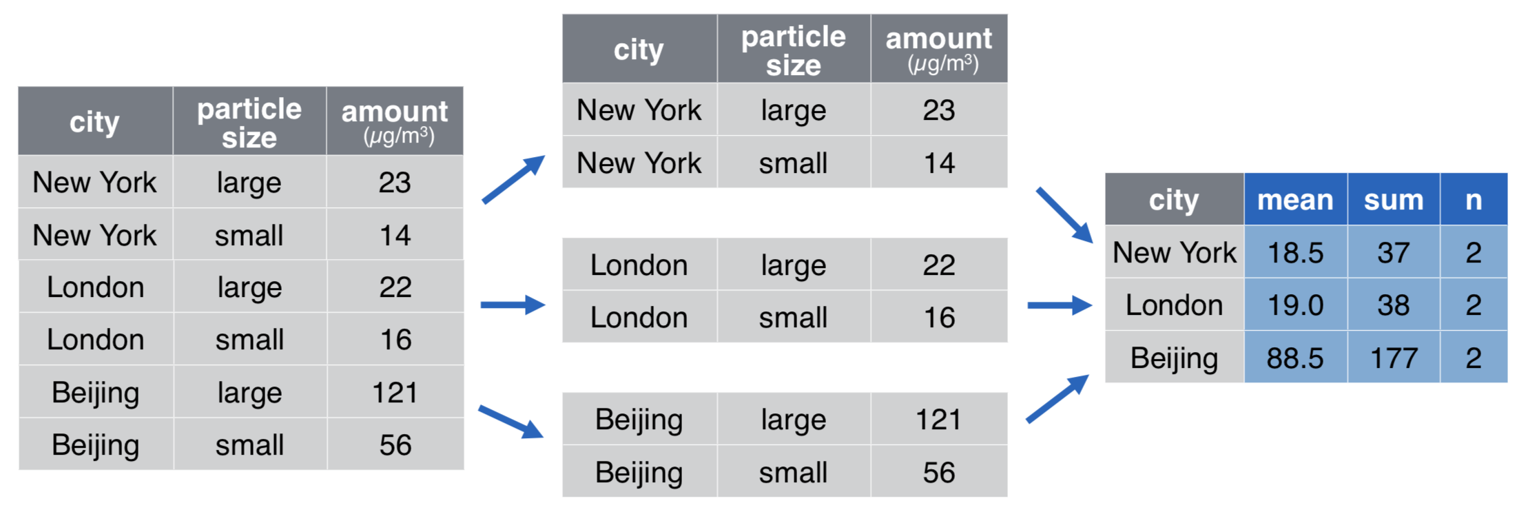
Statistics by group: `group_by` + `summarize`

Summary statistics by state

colleges %>%
  group_by(state) %>%
  summarize(
    n_schools = n(),
    avg_cost = mean(cost, na.rm = TRUE),
    min_size = min(undergrads, na.rm = TRUE),
    max_size = max(undergrads, na.rm = TRUE)
  )

# A tibble: 44 × 5
   state n_schools avg_cost min_size max_size
   <chr>     <int>    <dbl>    <dbl>    <dbl>
 1 AL            4   22242.      245     7785
 2 AR            3   43816.      512     1447
 3 AZ            2   33388.      803    33715
 4 CA            9   42807.       43    23337
 5 CO            2   45574      5755     8448
 6 CT            3   29895.      174     4425
 7 FL            5   34747.       39     2401
 8 GA            6   27961       235     9742
 9 HI            1   36765      1558     1558
10 IA            1     NaN       339      339
# ℹ 34 more rows

Your turn

Use group_by(), summarize(), and slice_max() to display the five dest airports with the most flights from NYC airports in 2023. Your display should include the median flight delay for these airports along with the number of flights to each airport.

03:30

Calculating counts

count() can be used as a short cut to group_by() + summarize() if you are only calculating counts

group_by()
count()

colleges %>% 
  group_by(state) %>%
  summarize(n = n())

# A tibble: 44 × 2
   state     n
   <chr> <int>
 1 AL        4
 2 AR        3
 3 AZ        2
 4 CA        9
 5 CO        2
 6 CT        3
 7 FL        5
 8 GA        6
 9 HI        1
10 IA        1
# ℹ 34 more rows

colleges %>% count(state)

# A tibble: 44 × 2
   state     n
   <chr> <int>
 1 AL        4
 2 AR        3
 3 AZ        2
 4 CA        9
 5 CO        2
 6 CT        3
 7 FL        5
 8 GA        6
 9 HI        1
10 IA        1
# ℹ 34 more rows

Calculations by group: `group_by` + `mutate`

Calculate z-scores within regions

colleges %>%
  group_by(region) %>%
  mutate(z_cost = (cost - mean(cost, na.rm = TRUE)) / sd(cost, na.rm = TRUE)) %>%
  relocate(unitid:region, z_cost, everything())

# A tibble: 187 × 14
# Groups:   region [10]
   unitid school type  city  state region z_cost admission_rate   act undergrads
    <dbl> <chr>  <chr> <chr> <chr> <chr>   <dbl>          <dbl> <dbl>      <dbl>
 1 228343 South… priv… Geor… TX    South…  1.51           0.490    26       1507
 2 177719 Barne… priv… Sain… MO    Plains NA             NA        NA        569
 3 367884 Hodge… priv… Fort… FL    South… -0.467          0.612    NA        832
 4 149781 Wheat… priv… Whea… IL    Great…  1.06           0.848    29       2358
 5 135364 Luthe… priv… Lith… GA    South… NA              0.5      NA        235
 6 212601 Ganno… priv… Erie  PA    Mid E…  0.261          0.755    23       2866
 7 133979 Flori… priv… Miam… FL    South… -0.465          0.400    NA       1049
 8 117140 Unive… priv… La V… CA    Far W…  1.14           0.548    22       4516
 9 152567 Trine… priv… Ango… IN    Great…  0.849          0.816    25       2120
10 237057 Whitm… priv… Wall… WA    Far W…  1.79           0.559    31       1545
# ℹ 177 more rows
# ℹ 4 more variables: cost <dbl>, grad_rate <dbl>, fy_retention <dbl>,
#   fedloan <dbl>

`ungroup()`

Once data are grouped, they remain grouped until you manually ungroup them
Some summary functions ungroup them for you, e.g., count() and summarize()

colleges %>%
  group_by(region) %>%
  mutate(z_cost = (cost - mean(cost, na.rm = TRUE)) / sd(cost, na.rm = TRUE)) %>%
  ungroup() %>%
  select(school, city, cost, z_cost)

With ungroup()
Without ungroup()

# A tibble: 187 × 4
   school                                           city           cost z_cost
   <chr>                                            <chr>         <dbl>  <dbl>
 1 Southwestern University                          Georgetown    55886  1.51 
 2 Barnes-Jewish College Goldfarb School of Nursing Saint Louis      NA NA    
 3 Hodges University                                Fort Myers    27425 -0.467
 4 Wheaton College                                  Wheaton       49214  1.06 
 5 Luther Rice College & Seminary                   Lithonia         NA NA    
 6 Gannon University                                Erie          44896  0.261
 7 Florida Memorial University                      Miami Gardens 27460 -0.465
 8 University of La Verne                           La Verne      58014  1.14 
 9 Trine University                                 Angola        46440  0.849
10 Whitman College                                  Walla Walla   68082  1.79 
# ℹ 177 more rows

# A tibble: 187 × 5
# Groups:   region [10]
   region      school                                         city   cost z_cost
   <chr>       <chr>                                          <chr> <dbl>  <dbl>
 1 Southwest   Southwestern University                        Geor… 55886  1.51 
 2 Plains      Barnes-Jewish College Goldfarb School of Nurs… Sain…    NA NA    
 3 Southeast   Hodges University                              Fort… 27425 -0.467
 4 Great Lakes Wheaton College                                Whea… 49214  1.06 
 5 Southeast   Luther Rice College & Seminary                 Lith…    NA NA    
 6 Mid East    Gannon University                              Erie  44896  0.261
 7 Southeast   Florida Memorial University                    Miam… 27460 -0.465
 8 Far West    University of La Verne                         La V… 58014  1.14 
 9 Great Lakes Trine University                               Ango… 46440  0.849
10 Far West    Whitman College                                Wall… 68082  1.79 
# ℹ 177 more rows

Aside: code commenting

In R, you can use # for adding comments to your code. Any text that follows the # will be printed as-is and won’t be run as code. This is useful for leaving comments in your code and for temporarily disabling certain lines of code for debugging.

colleges %>%
  group_by(state) %>%
  summarize(
    n_schools = n(),                               # This is a reminder to me
    # avg_cost = mean(cost, na.rm = TRUE),         # This line isn't run
    min_size = min(undergrads, na.rm = TRUE),
    max_size = max(undergrads, na.rm = TRUE)
  )

# A tibble: 44 × 4
   state n_schools min_size max_size
   <chr>     <int>    <dbl>    <dbl>
 1 AL            4      245     7785
 2 AR            3      512     1447
 3 AZ            2      803    33715
 4 CA            9       43    23337
 5 CO            2     5755     8448
 6 CT            3      174     4425
 7 FL            5       39     2401
 8 GA            6      235     9742
 9 HI            1     1558     1558
10 IA            1      339      339
# ℹ 34 more rows

Aside: code commenting

And it works especially well when you’ve used chaining in your code

colleges %>%
  #group_by(state) %>%
  summarize(
    n_schools = n(),                               
    avg_cost = mean(cost, na.rm = TRUE),         
    min_size = min(undergrads, na.rm = TRUE),
    max_size = max(undergrads, na.rm = TRUE)
  )

# A tibble: 1 × 4
  n_schools avg_cost min_size max_size
      <int>    <dbl>    <dbl>    <dbl>
1       187   36620.        0    33715

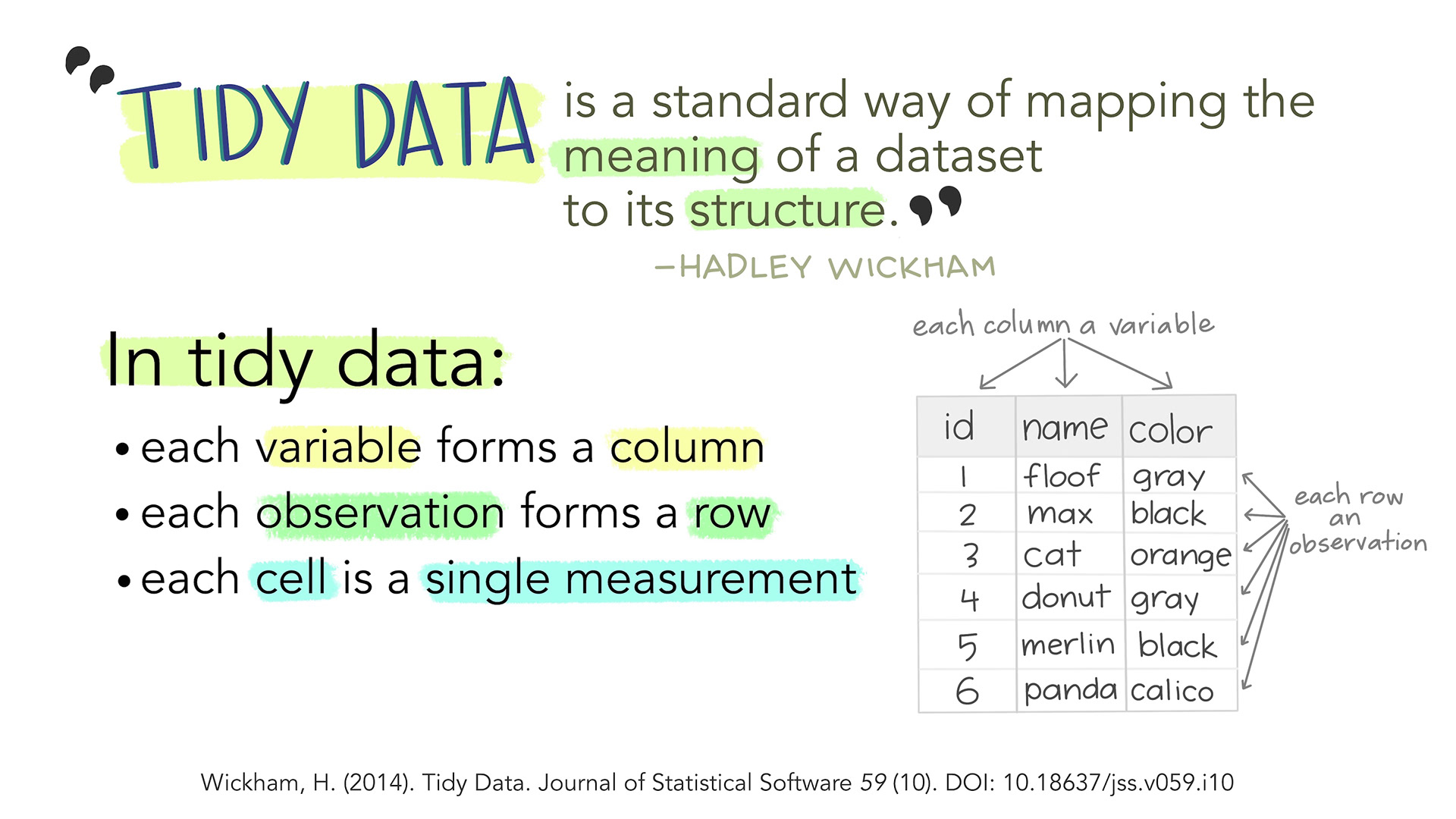
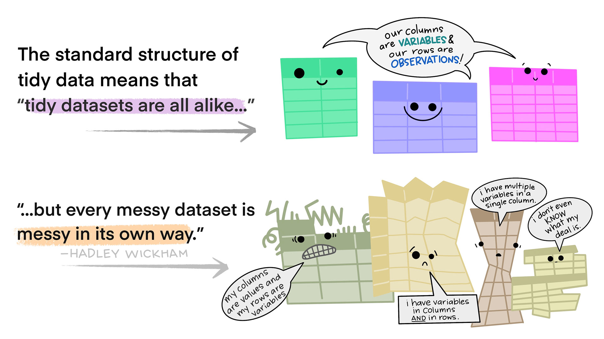
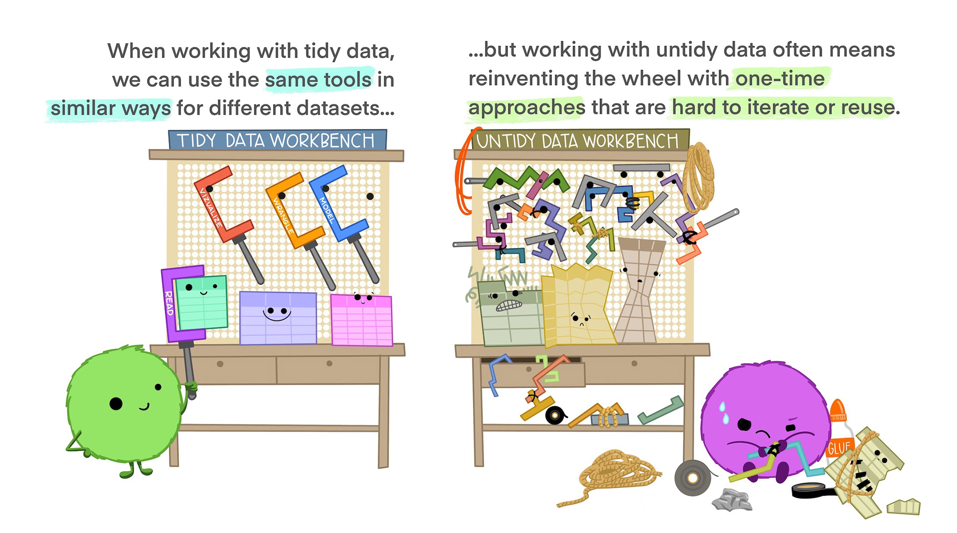
Intro to tidy data

Bakeoff ratings

Ratings data for each episode in series 1-8 (in millions of viewers)

# A tibble: 8 × 11
  series    e1    e2    e3    e4    e5    e6    e7    e8    e9   e10
   <dbl> <dbl> <dbl> <dbl> <dbl> <dbl> <dbl> <dbl> <dbl> <dbl> <dbl>
1      1  2.24  3     3     2.6   3.03  2.75 NA    NA    NA    NA   
2      2  3.1   3.53  3.82  3.6   3.83  4.25  4.42  5.06 NA    NA   
3      3  3.85  4.6   4.53  4.71  4.61  4.82  5.1   5.35  5.7   6.74
4      4  6.6   6.65  7.17  6.82  6.95  7.32  7.76  7.41  7.41  9.45
5      5  8.51  8.79  9.28 10.2   9.95 10.1  10.3   9.02 10.7  13.5 
6      6 11.6  11.6  12.0  12.4  12.4  12    12.4  11.1  12.6  15.0 
7      7 13.6  13.4  13.0  13.3  13.1  13.1  13.4  13.3  13.4  15.9 
8      8  9.46  9.23  8.68  8.55  8.61  8.61  9.01  8.95  9.03 10.0

Discuss

Is this dataset in tidy format? Why or why not?

If not, what would a tidy data set look like? Sketch out the first few rows of this data set in tidy format

02:00

`{tidyr}`

Reshape the layout of tabular data
Part of the tidyverse

Goal

Goal

Want to reshape the data to be in tidy format:

Current
Target

# A tibble: 8 × 11
  series    e1    e2    e3    e4    e5    e6    e7    e8    e9   e10
   <dbl> <dbl> <dbl> <dbl> <dbl> <dbl> <dbl> <dbl> <dbl> <dbl> <dbl>
1      1  2.24  3     3     2.6   3.03  2.75 NA    NA    NA    NA   
2      2  3.1   3.53  3.82  3.6   3.83  4.25  4.42  5.06 NA    NA   
3      3  3.85  4.6   4.53  4.71  4.61  4.82  5.1   5.35  5.7   6.74
4      4  6.6   6.65  7.17  6.82  6.95  7.32  7.76  7.41  7.41  9.45
5      5  8.51  8.79  9.28 10.2   9.95 10.1  10.3   9.02 10.7  13.5 
6      6 11.6  11.6  12.0  12.4  12.4  12    12.4  11.1  12.6  15.0 
7      7 13.6  13.4  13.0  13.3  13.1  13.1  13.4  13.3  13.4  15.9 
8      8  9.46  9.23  8.68  8.55  8.61  8.61  9.01  8.95  9.03 10.0

# A tibble: 80 × 3
   series epsiode rating
    <dbl> <chr>    <dbl>
 1      1 e1        2.24
 2      1 e2        3   
 3      1 e3        3   
 4      1 e4        2.6 
 5      1 e5        3.03
 6      1 e6        2.75
 7      1 e7       NA   
 8      1 e8       NA   
 9      1 e9       NA   
10      1 e10      NA   
# ℹ 70 more rows

`pivot_longer()`

data (as usual)

pivot_longer(
  data, 
  cols, 
  names_to = "name", 
  values_to = "value"
  )

`pivot_longer()`

data (as usual)
cols: columns to pivot into longer format

pivot_longer(
  data, 
  cols, 
  names_to = "name", 
  values_to = "value"
  )

`pivot_longer()`

data (as usual)
cols: columns to pivot into longer format
names_to: name of the column where column names of pivoted variables go (character string)

pivot_longer(
  data, 
  cols, 
  names_to = "name", 
  values_to = "value"
  )

`pivot_longer()`

data (as usual)
cols: columns to pivot into longer format
names_to: name of the column where column names of pivoted variables go (character string)
values_to: name of the column where data in pivoted variables go (character string)

pivot_longer(
  data, 
  cols, 
  names_to = "name", 
  values_to = "value"
  )

wider \(\rightarrow\) longer ratings

longer_ratings <- bakeoff_ratings %>%
  pivot_longer( 
    cols = e1:e10, 
    names_to = "episode", 
    values_to = "rating" 
  )
longer_ratings

# A tibble: 80 × 3
   series episode rating
    <dbl> <chr>    <dbl>
 1      1 e1        2.24
 2      1 e2        3   
 3      1 e3        3   
 4      1 e4        2.6 
 5      1 e5        3.03
 6      1 e6        2.75
 7      1 e7       NA   
 8      1 e8       NA   
 9      1 e9       NA   
10      1 e10      NA   
# ℹ 70 more rows

`parse_number()`

ratings <- longer_ratings %>%
  mutate(
    episode = parse_number(episode) 
  )
ratings

# A tibble: 80 × 3
   series episode rating
    <dbl>   <dbl>  <dbl>
 1      1       1   2.24
 2      1       2   3   
 3      1       3   3   
 4      1       4   2.6 
 5      1       5   3.03
 6      1       6   2.75
 7      1       7  NA   
 8      1       8  NA   
 9      1       9  NA   
10      1      10  NA   
# ℹ 70 more rows

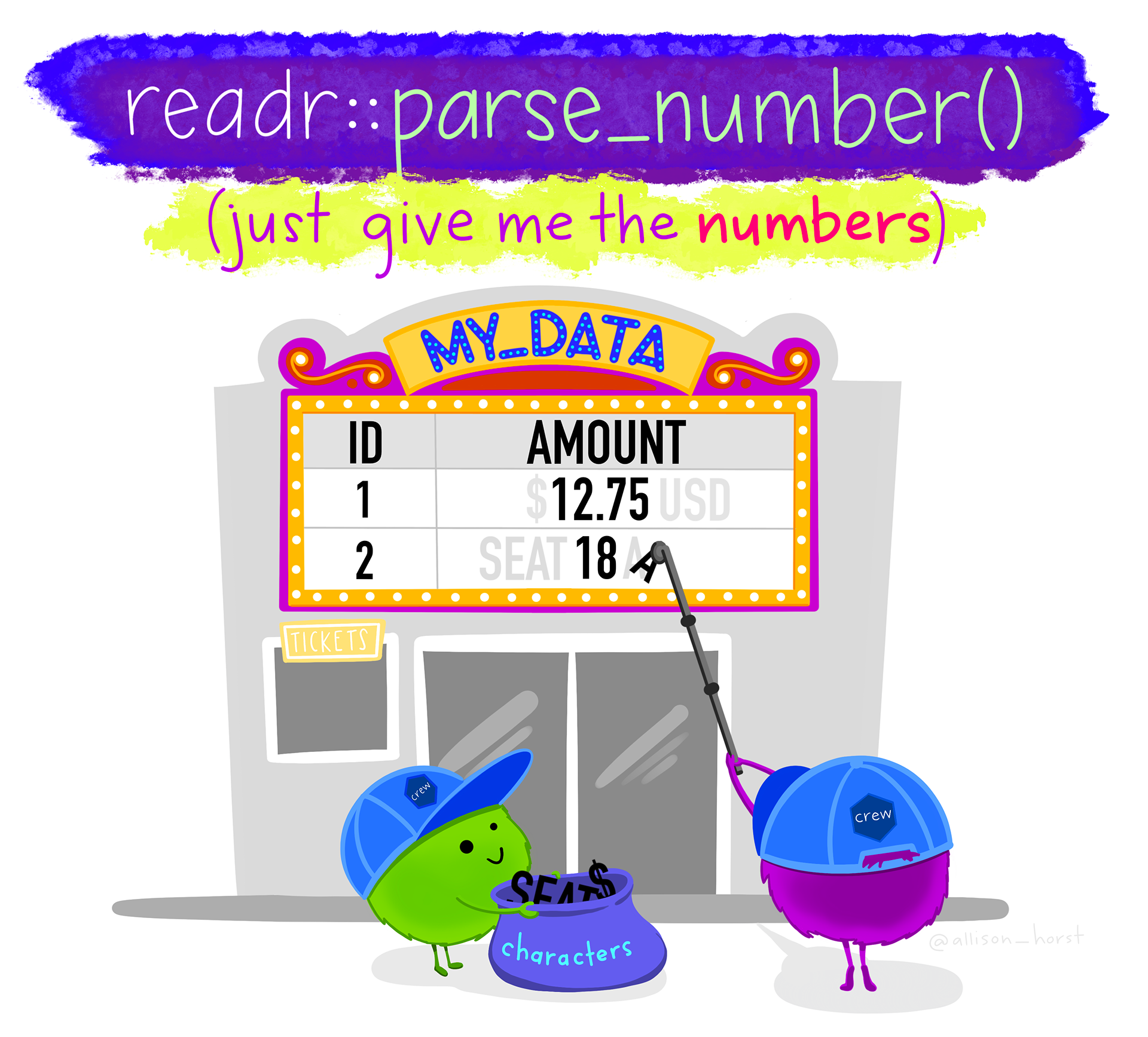
Other parsing functions

parse_character

parse_date

parse_double

parse_factor

parse_integer

parse_logical

parse_number

parse_time

Try it: `messy_ratings`

Tidy this data set by

Selecting the series and e*_7day columns
Pivoting the data to add a column for episode and a column for rating (we’ll clean up the episode column later)

messy_ratings2 <- read_csv("https://stat220-s25.github.io/data/messy_ratings2.csv")
messy_ratings2

# A tibble: 8 × 21
  series e1_7day e1_28day e2_7day e2_28day e3_7day e3_28day e4_7day e4_28day
   <dbl>   <dbl>    <dbl>   <dbl>    <dbl>   <dbl>    <dbl>   <dbl>    <dbl>
1      1    2.24    NA       3       NA       3       NA       2.6     NA   
2      2    3.1     NA       3.53    NA       3.82    NA       3.6     NA   
3      3    3.85    NA       4.6     NA       4.53    NA       4.71    NA   
4      4    6.6     NA       6.65    NA       7.17    NA       6.82    NA   
5      5    8.51    NA       8.79    NA       9.28    NA      10.2     NA   
6      6   11.6     11.7    11.6     11.8    12.0     NA      12.4     12.7 
7      7   13.6     13.9    13.4     13.7    13.0     13.4    13.3     13.9 
8      8    9.46     9.72    9.23     9.53    8.68     9.06    8.55     8.87
# ℹ 12 more variables: e5_7day <dbl>, e5_28day <dbl>, e6_7day <dbl>,
#   e6_28day <dbl>, e7_7day <dbl>, e7_28day <dbl>, e8_7day <dbl>,
#   e8_28day <dbl>, e9_7day <dbl>, e9_28day <dbl>, e10_7day <dbl>,
#   e10_28day <dbl>

04:00

Cleaning `episode`

ratings2 <- messy_ratings2 %>%
  select(series, contains("7day")) %>%
  pivot_longer(contains("7day"), 
               names_to = "episode", 
               values_to = "rating")
ratings2

# A tibble: 80 × 3
   series episode  rating
    <dbl> <chr>     <dbl>
 1      1 e1_7day    2.24
 2      1 e2_7day    3   
 3      1 e3_7day    3   
 4      1 e4_7day    2.6 
 5      1 e5_7day    3.03
 6      1 e6_7day    2.75
 7      1 e7_7day   NA   
 8      1 e8_7day   NA   
 9      1 e9_7day   NA   
10      1 e10_7day  NA   
# ℹ 70 more rows

`separate()`

data (as usual)

separate(
  data, 
  col, 
  into = c("col1", "col2"),
  sep 
  )

`separate()`

data (as usual)
col: column to separate

separate(
  data, 
  col, 
  into = c("col1", "col2"),
  sep 
  )

`separate()`

data (as usual)
col: column to separate
into: names of new columns to create

separate(
  data, 
  col, 
  into = c("col1", "col2"),
  sep 
  )

`separate()`

data (as usual)
col: column to separate
into: names of new columns to create
sep: separator between columns

separate(
  data, 
  col, 
  into = c("col1", "col2"),
  sep 
  )

Cleaning `episode`

ratings2 %>%
  separate( 
    col = episode, 
    into = c("episode", "period") 
  )

# A tibble: 80 × 4
   series episode period rating
    <dbl> <chr>   <chr>   <dbl>
 1      1 e1      7day     2.24
 2      1 e2      7day     3   
 3      1 e3      7day     3   
 4      1 e4      7day     2.6 
 5      1 e5      7day     3.03
 6      1 e6      7day     2.75
 7      1 e7      7day    NA   
 8      1 e8      7day    NA   
 9      1 e9      7day    NA   
10      1 e10     7day    NA   
# ℹ 70 more rows

Wrap it up

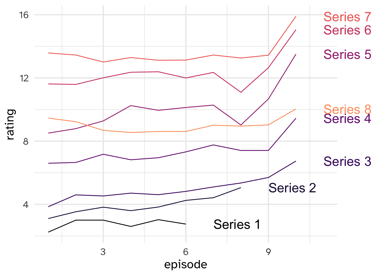
Clean the episode and period column
Make a line plot with episode on the x-axis, rating on the y-axis, colored by series. (You will also need to map the group aesthetic to series)

Data Wrangling: Groups & Tidy Data

The College Scorecard

Using %>% or |>

The |> (base) pipe

Calculating Summaries

Computing statistics: summarize

Computing statistics: summarize

Your turn

Your turn

group_by()

Spit-apply-combine

Statistics by group: group_by + summarize

Your turn

Calculating counts

Calculations by group: group_by + mutate

ungroup()

Aside: code commenting

Aside: code commenting

Intro to tidy data

Bakeoff ratings

Discuss

{tidyr}

Goal

Goal

pivot_longer()

pivot_longer()

pivot_longer()

pivot_longer()

wider \(\rightarrow\) longer ratings

parse_number()

Other parsing functions

Try it: messy_ratings

Cleaning episode

separate()

separate()

separate()

separate()

Cleaning episode

Wrap it up

Data Wrangling:
Groups &
Tidy Data

Using `%>%` or `|>`

The `|>` (base) pipe

Computing statistics: `summarize`

Computing statistics: `summarize`

`group_by()`

Statistics by group: `group_by` + `summarize`

Calculations by group: `group_by` + `mutate`

`ungroup()`

`{tidyr}`

`pivot_longer()`

`pivot_longer()`

`pivot_longer()`

`pivot_longer()`

`parse_number()`

Try it: `messy_ratings`

Cleaning `episode`

`separate()`

`separate()`

`separate()`

`separate()`

Cleaning `episode`