Data Wrangling:
Combining Data

Day 10

Prof Amanda Luby

Carleton College
Stat 220 - Spring 2025

Today

Peer programming

Work on code in a small group (2-3)
One person does the typing, the others observe and support
Rules of thumb:
- no typing until your group has discussed a possible approach
- let the typer finish their command/line/pipeline before pointing out any typos
- everybody should contribute ideas and understand the code that is written
Whoever does the typing will share the completed .Rmd so you all have it

Warm up

Find your groupmates, introduce yourselves:
- Name & topic of your first portfolio project
Choose someone to be the “typer”. That person should open the 10-combining.rmd activity in RStudio
- Can’t decide? Choose the person who had the shortest walk to class today
Take a look at the first 3 pairs of data together and talk through (conceptually! in words!) how you think they should be combined

08:00

Example 1: Star Wars Characters

Dataset 1:

starwars_characters

# A tibble: 87 × 6
   name               height  mass homeworld species first_film
   <chr>               <int> <dbl> <chr>     <chr>   <chr>     
 1 Luke Skywalker        172    77 Tatooine  Human   A New Hope
 2 C-3PO                 167    75 Tatooine  Droid   A New Hope
 3 R2-D2                  96    32 Naboo     Droid   A New Hope
 4 Darth Vader           202   136 Tatooine  Human   A New Hope
 5 Leia Organa           150    49 Alderaan  Human   A New Hope
 6 Owen Lars             178   120 Tatooine  Human   A New Hope
 7 Beru Whitesun Lars    165    75 Tatooine  Human   A New Hope
 8 R5-D4                  97    32 Tatooine  Droid   A New Hope
 9 Biggs Darklighter     183    84 Tatooine  Human   A New Hope
10 Obi-Wan Kenobi        182    77 Stewjon   Human   A New Hope
# ℹ 77 more rows

Dataset 2:

starwars_lastjedi

# A tibble: 2 × 6
  name         height mass  homeworld species first_film   
  <chr>        <lgl>  <lgl> <chr>     <chr>   <chr>        
1 Rose Tico    NA     NA    Otomok    Human   The Last Jedi
2 Amilyn Holdo NA     NA    <NA>      Human   The Last Jedi

`bind_rows()`

data_1: our “starting” data
data_2 to data_n: additional rows of data that we want to add to data_1

bind_rows(
  data_1, 
  data_2, 
  ..., 
  data_n
  )

starwars_characters %>%
  bind_rows(starwars_lastjedi) %>%
  slice_tail(n=10)

# A tibble: 10 × 6
   name            height  mass homeworld species first_film          
   <chr>            <int> <dbl> <chr>     <chr>   <chr>               
 1 Raymus Antilles    188    79 Alderaan  Human   A New Hope          
 2 Sly Moore          178    48 Umbara    <NA>    Attack of the Clones
 3 Tion Medon         206    80 Utapau    Pau'an  Revenge of the Sith 
 4 Finn                NA    NA <NA>      Human   The Force Awakens   
 5 Rey                 NA    NA <NA>      Human   The Force Awakens   
 6 Poe Dameron         NA    NA <NA>      Human   The Force Awakens   
 7 BB8                 NA    NA <NA>      Droid   The Force Awakens   
 8 Captain Phasma      NA    NA <NA>      Human   The Force Awakens   
 9 Rose Tico           NA    NA Otomok    Human   The Last Jedi       
10 Amilyn Holdo        NA    NA <NA>      Human   The Last Jedi

Example 2: Stats Sections

Dataset 1:

stats_sections_fw

# A tibble: 8 × 3
  class    fall winter
  <chr>   <dbl>  <dbl>
1 stat120     3      3
2 stat220     1      1
3 stat230     1      1
4 stat250     0      1
5 stat270     1      0
6 stat285     1      1
7 stat320     0      0
8 stat330     0      1

Dataset 2:

stats_sections_s

# A tibble: 8 × 1
  spring
   <dbl>
1      4
2      1
3      1
4      1
5      0
6      1
7      1
8      0

`bind_cols()`

data_1: our “starting” data
data_2 to data_n: additional columns of data that we want to add to data_1

bind_cols(
  data_1, 
  data_2, 
  ..., 
  data_n
  )

stats_sections_fw %>%
  bind_cols(stats_sections_s)

# A tibble: 8 × 4
  class    fall winter spring
  <chr>   <dbl>  <dbl>  <dbl>
1 stat120     3      3      4
2 stat220     1      1      1
3 stat230     1      1      1
4 stat250     0      1      1
5 stat270     1      0      0
6 stat285     1      1      1
7 stat320     0      0      1
8 stat330     0      1      0

We got lucky

Our second dataset followed this structure:

# A tibble: 8 × 2
  class   spring
  <chr>    <dbl>
1 stat120      4
2 stat220      1
3 stat230      1
4 stat250      1
5 stat270      0
6 stat285      1
7 stat320      1
8 stat330      0

But it could have also had this structure:

# A tibble: 8 × 2
  class   spring
  <chr>    <dbl>
1 stat270      0
2 stat330      0
3 stat220      1
4 stat230      1
5 stat250      1
6 stat285      1
7 stat320      1
8 stat120      4

Example 3: Survivor castaways

Dataset 1:

us_castaway_results

# A tibble: 870 × 7
   castaway_id castaway season_name      season place jury  finalist
   <chr>       <chr>    <chr>             <dbl> <dbl> <lgl> <lgl>   
 1 US0001      Sonja    Survivor: Borneo      1    16 FALSE FALSE   
 2 US0002      B.B.     Survivor: Borneo      1    15 FALSE FALSE   
 3 US0003      Stacey   Survivor: Borneo      1    14 FALSE FALSE   
 4 US0004      Ramona   Survivor: Borneo      1    13 FALSE FALSE   
 5 US0005      Dirk     Survivor: Borneo      1    12 FALSE FALSE   
 6 US0006      Joel     Survivor: Borneo      1    11 FALSE FALSE   
 7 US0007      Gretchen Survivor: Borneo      1    10 FALSE FALSE   
 8 US0008      Greg     Survivor: Borneo      1     9 TRUE  FALSE   
 9 US0009      Jenna    Survivor: Borneo      1     8 TRUE  FALSE   
10 US0010      Gervase  Survivor: Borneo      1     7 TRUE  FALSE   
# ℹ 860 more rows

Dataset 2:

cast_details

# A tibble: 1,118 × 6
   castaway_id full_name        date_of_birth gender occupation personality_type
   <chr>       <chr>            <date>        <chr>  <chr>      <chr>           
 1 US0014      Rudy Boesch      1928-01-20    Male   Retired N… ISTJ            
 2 US0002      B.B. Andersen    1936-01-18    Male   Real Esta… ESTJ            
 3 US0001      Sonja Christoph… 1937-01-28    Female Musician   ENFP            
 4 US0075      Jake Billingsley 1941-08-21    Male   Land Brok… ISFJ            
 5 US0151      Jim Lynch        1942-01-07    Male   Retired F… ISTJ            
 6 US0474      Joseph Del Campo 1943-07-04    Male   Former FB… ISTJ            
 7 US0304      Jimmy Johnson    1943-07-16    Male   Former NF… ESFJ            
 8 US0047      Kim Johnson      1944-09-18    Female Retired T… ISFJ            
 9 US0128      Scout Cloud Lee  1944-11-08    Female Rancher    INFJ            
10 US0061      Paschal English  1945-03-05    Male   Judge      ISFJ            
# ℹ 1,108 more rows

Desired output

# A tibble: 870 × 12
   castaway_id castaway season_name      season place jury  finalist full_name  
   <chr>       <chr>    <chr>             <dbl> <dbl> <lgl> <lgl>    <chr>      
 1 US0001      Sonja    Survivor: Borneo      1    16 FALSE FALSE    Sonja Chri…
 2 US0002      B.B.     Survivor: Borneo      1    15 FALSE FALSE    B.B. Ander…
 3 US0003      Stacey   Survivor: Borneo      1    14 FALSE FALSE    Stacey Sti…
 4 US0004      Ramona   Survivor: Borneo      1    13 FALSE FALSE    Ramona Gray
 5 US0005      Dirk     Survivor: Borneo      1    12 FALSE FALSE    Dirk Been  
 6 US0006      Joel     Survivor: Borneo      1    11 FALSE FALSE    Joel Klug  
 7 US0007      Gretchen Survivor: Borneo      1    10 FALSE FALSE    Gretchen C…
 8 US0008      Greg     Survivor: Borneo      1     9 TRUE  FALSE    Greg Buis  
 9 US0009      Jenna    Survivor: Borneo      1     8 TRUE  FALSE    Jenna Lewis
10 US0010      Gervase  Survivor: Borneo      1     7 TRUE  FALSE    Gervase Pe…
# ℹ 860 more rows
# ℹ 4 more variables: date_of_birth <date>, gender <chr>, occupation <chr>,
#   personality_type <chr>

`left_join()`

us_castaway_results %>%
  left_join(cast_details, by = "castaway_id") %>%
  select(-season_name)

# A tibble: 870 × 11
   castaway_id castaway season place jury  finalist full_name      date_of_birth
   <chr>       <chr>     <dbl> <dbl> <lgl> <lgl>    <chr>          <date>       
 1 US0001      Sonja         1    16 FALSE FALSE    Sonja Christo… 1937-01-28   
 2 US0002      B.B.          1    15 FALSE FALSE    B.B. Andersen  1936-01-18   
 3 US0003      Stacey        1    14 FALSE FALSE    Stacey Stillm… 1972-08-11   
 4 US0004      Ramona        1    13 FALSE FALSE    Ramona Gray    1971-01-20   
 5 US0005      Dirk          1    12 FALSE FALSE    Dirk Been      1976-06-15   
 6 US0006      Joel          1    11 FALSE FALSE    Joel Klug      1972-04-13   
 7 US0007      Gretchen      1    10 FALSE FALSE    Gretchen Cordy 1962-02-07   
 8 US0008      Greg          1     9 TRUE  FALSE    Greg Buis      1975-12-31   
 9 US0009      Jenna         1     8 TRUE  FALSE    Jenna Lewis    1977-07-16   
10 US0010      Gervase       1     7 TRUE  FALSE    Gervase Peter… 1969-11-02   
# ℹ 860 more rows
# ℹ 3 more variables: gender <chr>, occupation <chr>, personality_type <chr>

`left_join()` keeps duplicate rows in `x`

us_castaway_results %>%
  left_join(cast_details, by = "castaway_id") %>%
  filter(castaway == "Sandra") %>%
  select(-season_name)

# A tibble: 4 × 11
  castaway_id castaway season place jury  finalist full_name       date_of_birth
  <chr>       <chr>     <dbl> <dbl> <lgl> <lgl>    <chr>           <date>       
1 US0112      Sandra        7     1 FALSE TRUE     Sandra Diaz-Tw… 1974-07-30   
2 US0112      Sandra       20     1 FALSE TRUE     Sandra Diaz-Tw… 1974-07-30   
3 US0112      Sandra       34    15 FALSE FALSE    Sandra Diaz-Tw… 1974-07-30   
4 US0112      Sandra       40    15 FALSE FALSE    Sandra Diaz-Tw… 1974-07-30   
# ℹ 3 more variables: gender <chr>, occupation <chr>, personality_type <chr>

Other types of `_join`s

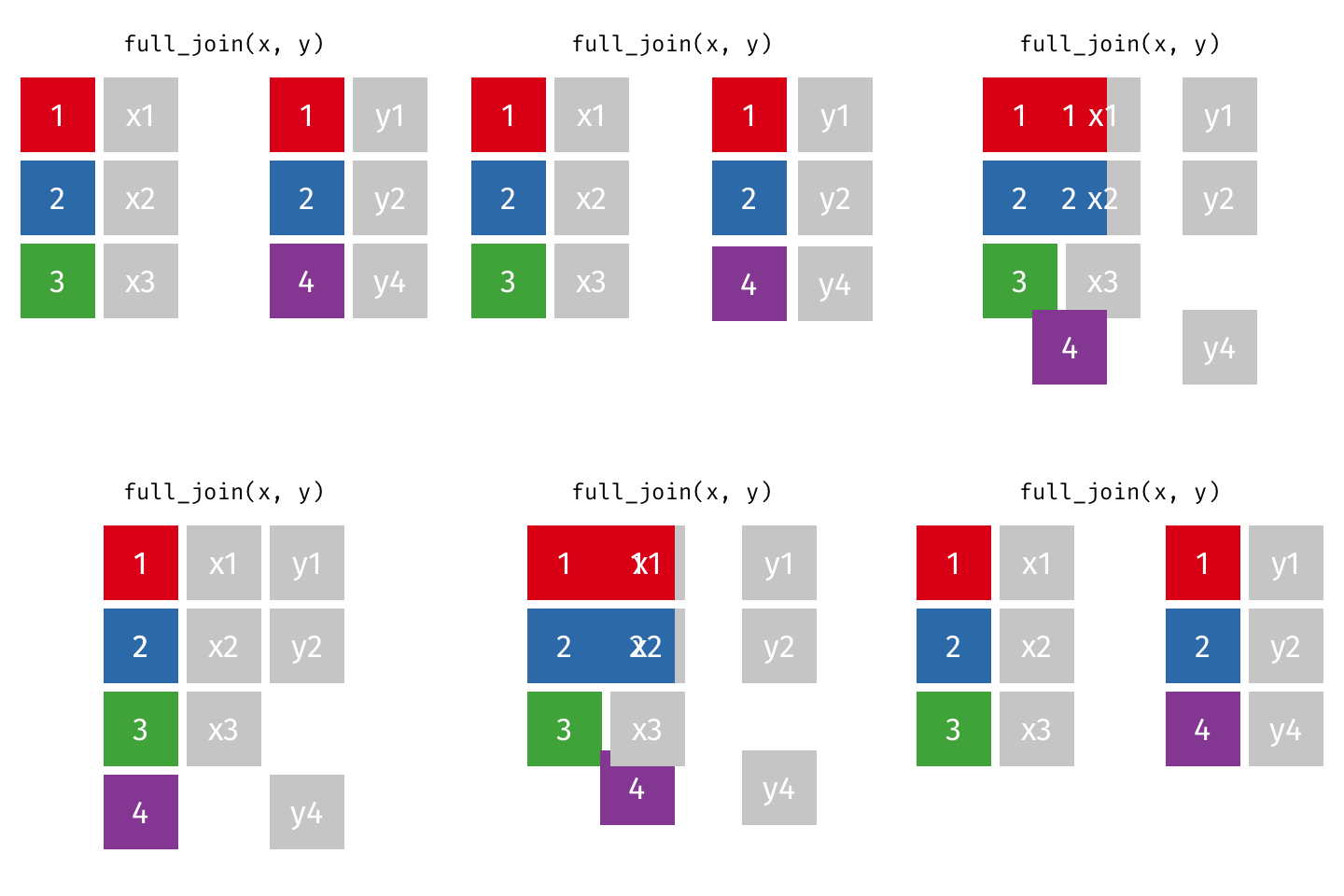
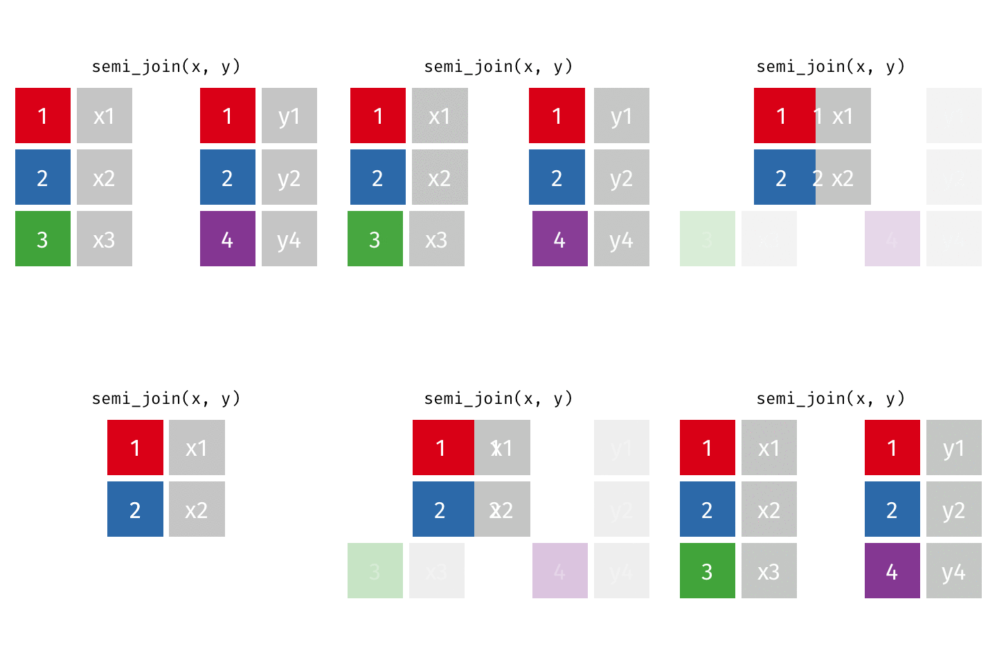
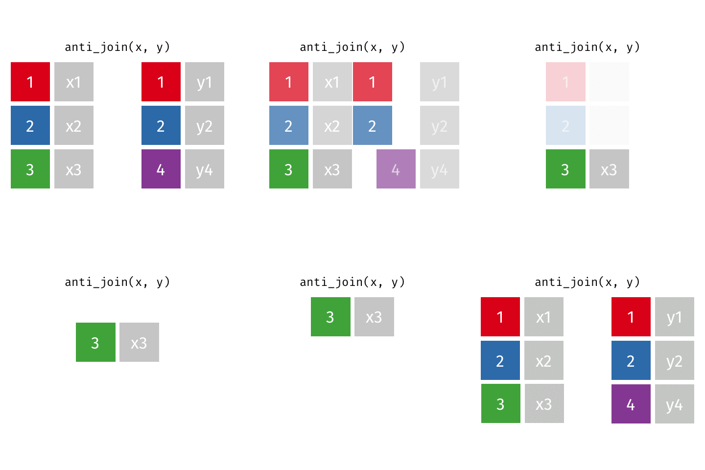
left_join(): all rows from x
right_join(): all rows from y
full_join(): all rows from both x and y
inner_join(): all rows from x where there are matching values in y, return all combination of multiple matches in the case of multiple matches
semi_join(): all rows from x where there are matching values in y, keeping just columns from x
anti_join(): return all rows from x where there are not matching values in y, never duplicate rows of x
…

Setup

For the next few slides…

# A tibble: 3 × 2
     id value_x
  <dbl> <chr>  
1     1 x1     
2     2 x2     
3     3 x3

# A tibble: 3 × 2
     id value_y
  <dbl> <chr>  
1     1 y1     
2     2 y2     
3     4 y4

`left_join()`

Keep all rows from x

left_join(x, y, by = "id")

# A tibble: 3 × 3
     id value_x value_y
  <dbl> <chr>   <chr>  
1     1 x1      y1     
2     2 x2      y2     
3     3 x3      <NA>

`full_join()`

Keep all rows from both x and y

full_join(x, y)

# A tibble: 4 × 3
     id value_x value_y
  <dbl> <chr>   <chr>  
1     1 x1      y1     
2     2 x2      y2     
3     3 x3      <NA>   
4     4 <NA>    y4

`semi_join()`

Keep all rows from x where there are matching values in y, keeping just columns from x

semi_join(x, y)

# A tibble: 2 × 2
     id value_x
  <dbl> <chr>  
1     1 x1     
2     2 x2

Similar to filter()

`anti_join()`

Keep all rows from x where there are not matching values in y, never duplicate rows of x

anti_join(x, y)

# A tibble: 1 × 2
     id value_x
  <dbl> <chr>  
1     3 x3

Similar to filter() with !

`*_join()` functions

From dplyr
Incredibly useful for bringing datasets with common information (e.g., unique identifier) together
Use by argument
Always check that the numbers of rows and columns of the result dataset makes sense
Refer to two-table verbs vignette when needed

keys

In these examples, the colored boxes represent keys

keys uniquely identify the observation of interest
Are present in both datasets and used to match the rows
Depend on the context (e.g. could be castaway ID, could be season ID, could be epiosde number, etc.)
Can be multiple columns
dplyr will try to find them automatically, but it’s better to be explicit using the by argument

Let’s try it: Bakeoff data (again)

On Friday, we tidied data containing ratings from The Great British Bakeoff.

Before:

# A tibble: 3 × 21
  series e1_7day e1_28day e2_7day e2_28day e3_7day e3_28day e4_7day e4_28day
   <dbl>   <dbl>    <dbl>   <dbl>    <dbl>   <dbl>    <dbl>   <dbl>    <dbl>
1      1    2.24       NA    3          NA    3          NA    2.6        NA
2      2    3.1        NA    3.53       NA    3.82       NA    3.6        NA
3      3    3.85       NA    4.6        NA    4.53       NA    4.71       NA
# ℹ 12 more variables: e5_7day <dbl>, e5_28day <dbl>, e6_7day <dbl>,
#   e6_28day <dbl>, e7_7day <dbl>, e7_28day <dbl>, e8_7day <dbl>,
#   e8_28day <dbl>, e9_7day <dbl>, e9_28day <dbl>, e10_7day <dbl>,
#   e10_28day <dbl>

After:

# A tibble: 5 × 4
  series episode period viewers
   <dbl>   <dbl>  <dbl>   <dbl>
1      1       1      7    2.24
2      1       2      7    3   
3      1       3      7    3   
4      1       4      7    2.6 
5      1       5      7    3.03

Let’s try it: Bakeoff data (again)

But that data only had through season 8. We now have a new dataset with seasons 9-14:

# A tibble: 6 × 21
  series e1_7day e1_28day e2_7day e2_28day e3_7day e3_28day e4_7day e4_28day
   <dbl>   <dbl>    <dbl>   <dbl>    <dbl>   <dbl>    <dbl>   <dbl>    <dbl>
1      9    9.55     9.92    9.31     9.76    8.91     9.35    8.88     9.41
2     10    9.62    10.0     9.38     9.8     8.94     9.42    8.96     9.49
3     11   11.2     11.8    10.8     11.4    10.7     11.2    10.6     11.2 
4     12    9.57    10.2     8.98     9.64    8.69     9.39    8.75     9.13
5     13    8.3      1       7.6      1       7.35     1       7.76     1   
6     14    7.84     1       7.54     1       7.28     1       7.12     1   
# ℹ 12 more variables: e5_7day <dbl>, e5_28day <dbl>, e6_7day <dbl>,
#   e6_28day <dbl>, e7_7day <dbl>, e7_28day <dbl>, e8_7day <dbl>,
#   e8_28day <dbl>, e9_7day <dbl>, e9_28day <dbl>, e10_7day <dbl>,
#   e10_28day <dbl>

Your task is to join these two datasets together using (1) bind_rows(), (2) _join() and (3) bind_cols() (you’ll also get some pivot_ practice along the way)

Part II: the `episodes` data

The episodes data has information about each episode of GBBO.

In particular, it includes:

baker: each baker that competed on that episode
signature: the name of the dessert they made for the signature challenge
technical: the place the baker earned in the technical challenge
showstopper: the name of the dessert they made for the showstopper challenge
result: whether the baker was “Safe” or “Eliminated”

episodes

# A tibble: 1,007 × 7
   series episode baker     signature               technical showstopper result
    <dbl>   <dbl> <chr>     <chr>                       <dbl> <chr>       <chr> 
 1      1       1 Annetha   Light Jamaican Black C…         2 Red, White… Safe  
 2      1       1 David     Chocolate Orange Cake           3 Black Fore… Safe  
 3      1       1 Edd       Caramel Cinnamon and B…         1 <NA>        Safe  
 4      1       1 Jasminder Fresh Mango and Passio…        NA <NA>        Safe  
 5      1       1 Jonathan  Carrot Cake with Lime …         9 Three Tier… Safe  
 6      1       1 Lea       Cranberry and Pistachi…        10 Raspberrie… Elimi…
 7      1       1 Louise    Carrot and Orange Cake         NA Never Fail… Safe  
 8      1       1 Mark      Sticky Marmalade Tea L…        NA Heart-shap… Elimi…
 9      1       1 Miranda   Triple Layered Brownie…         8 Three Tier… Safe  
10      1       1 Ruth      Lemon Drizzle Cakewith…        NA Classic Ch… Safe  
# ℹ 997 more rows

Let’s try it: Bakeoff data (episodes)

Join the tidy dataset (all 14 seasons) with the episodes data.

Your task is to print the “signature” desserts that were made on the 10 episodes that had the highest 7-day viewership.

Data Wrangling: Combining Data

Today

Peer programming

Warm up

Example 1: Star Wars Characters

bind_rows()

Example 2: Stats Sections

bind_cols()

We got lucky

Example 3: Survivor castaways

Desired output

left_join()

left_join() keeps duplicate rows in x

Other types of _joins

Setup

left_join()

full_join()

semi_join()

anti_join()

*_join() functions

keys

Let’s try it: Bakeoff data (again)

Let’s try it: Bakeoff data (again)

Part II: the episodes data

Let’s try it: Bakeoff data (episodes)

Data Wrangling:
Combining Data

`bind_rows()`

`bind_cols()`

`left_join()`

`left_join()` keeps duplicate rows in `x`

Other types of `_join`s

`left_join()`

`full_join()`

`semi_join()`

`anti_join()`

`*_join()` functions

Part II: the `episodes` data