# A tibble: 1,351 × 29
   version version_season season_name      season full_name castaway_id castaway
   <fct>   <chr>          <chr>             <dbl> <chr>     <chr>       <chr>
 1 US      US01           Survivor: Borneo      1 Sonja Ch… US0001      Sonja
 2 US      US01           Survivor: Borneo      1 B.B. And… US0002      B.B.
 3 US      US01           Survivor: Borneo      1 Stacey S… US0003      Stacey
 4 US      US01           Survivor: Borneo      1 Ramona G… US0004      Ramona
 5 US      US01           Survivor: Borneo      1 Dirk Been US0005      Dirk
 6 US      US01           Survivor: Borneo      1 Joel Klug US0006      Joel
 7 US      US01           Survivor: Borneo      1 Gretchen… US0007      Gretchen
 8 US      US01           Survivor: Borneo      1 Greg Buis US0008      Greg
 9 US      US01           Survivor: Borneo      1 Jenna Le… US0009      Jenna
10 US      US01           Survivor: Borneo      1 Gervase … US0010      Gervase
# ℹ 1,341 more rows
# ℹ 22 more variables: age <dbl>, city <chr>, state <chr>, episode <dbl>,
#   day <dbl>, order <dbl>, result <chr>, place <dbl>, jury_status <chr>,
#   original_tribe <chr>, jury <lgl>, finalist <lgl>, winner <lgl>,
#   acknowledge <lgl>, ack_look <lgl>, ack_speak <lgl>, ack_gesture <lgl>,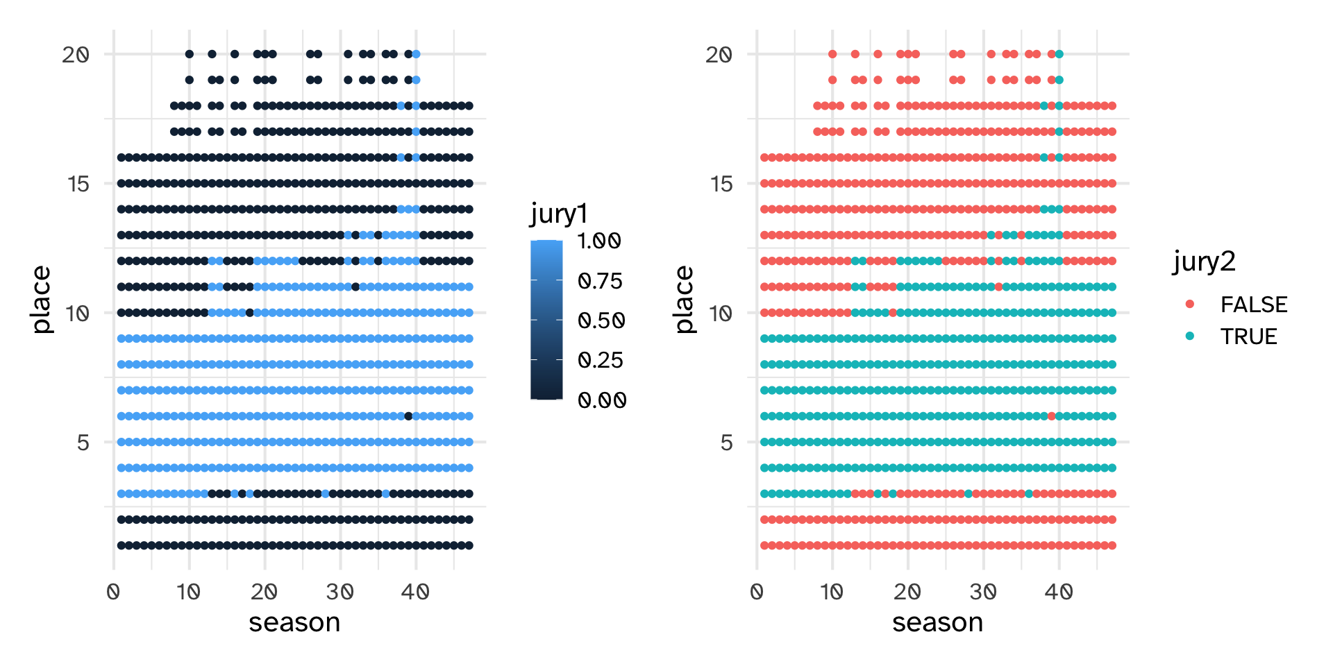
# ack_smile <lgl>, ack_quote <chr>, ack_score <dbl>, jury1 <dbl>, jury2 <fct>Working with
Factors
Day 12
Same graph, colored by the same categorical variable
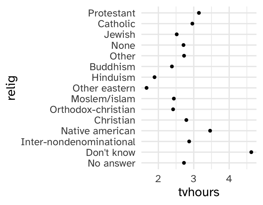
Which religions watch the least TV?
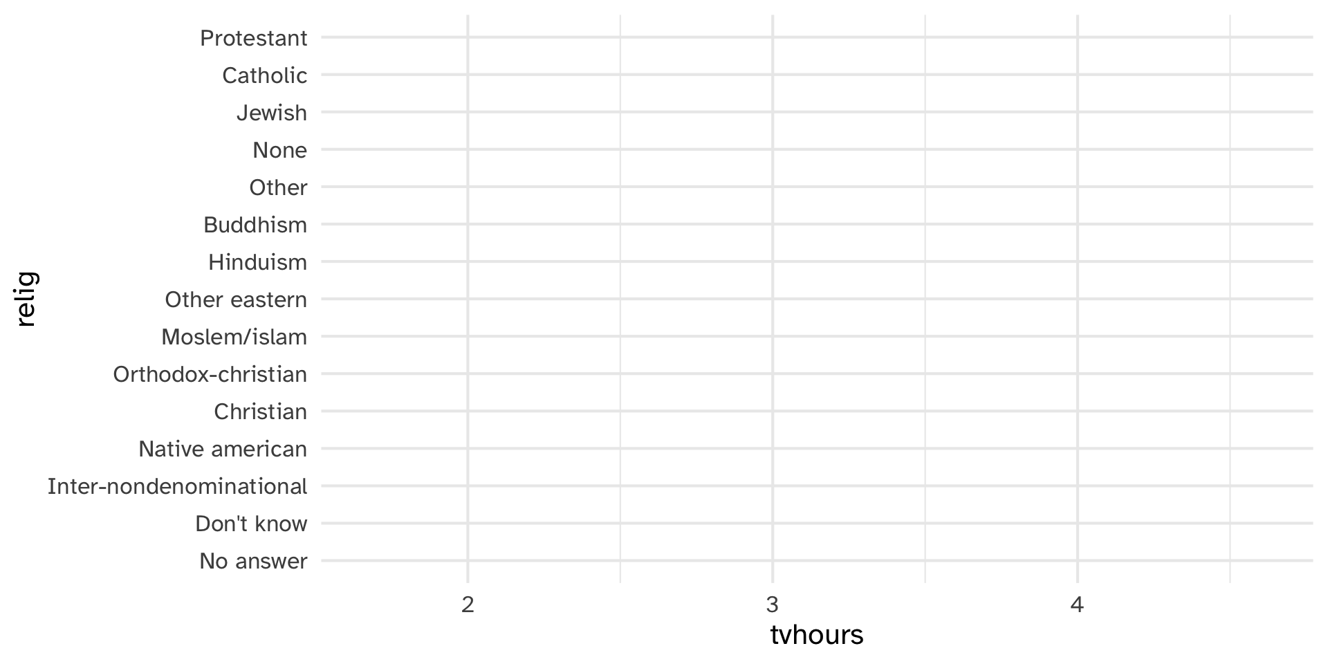
Which religions watch the least TV?
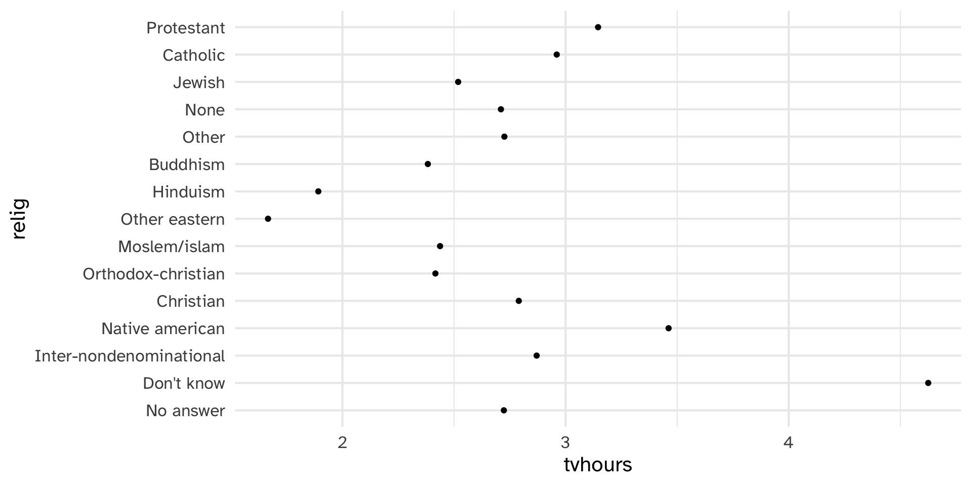
Which do you prefer?
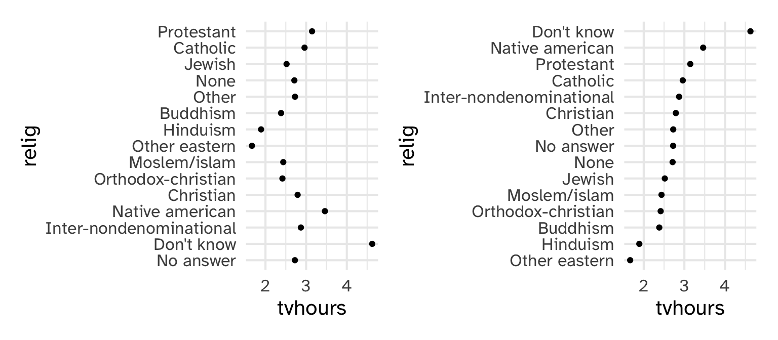
Why is the y-axis in this order?
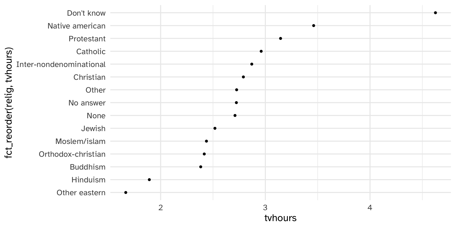
Reorder relig by tvhours

Reorder relig by tvhours
Which do you prefer?
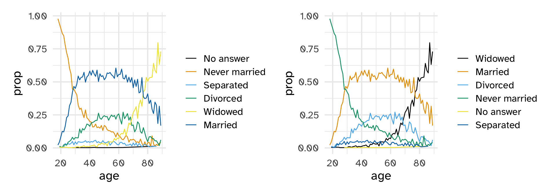
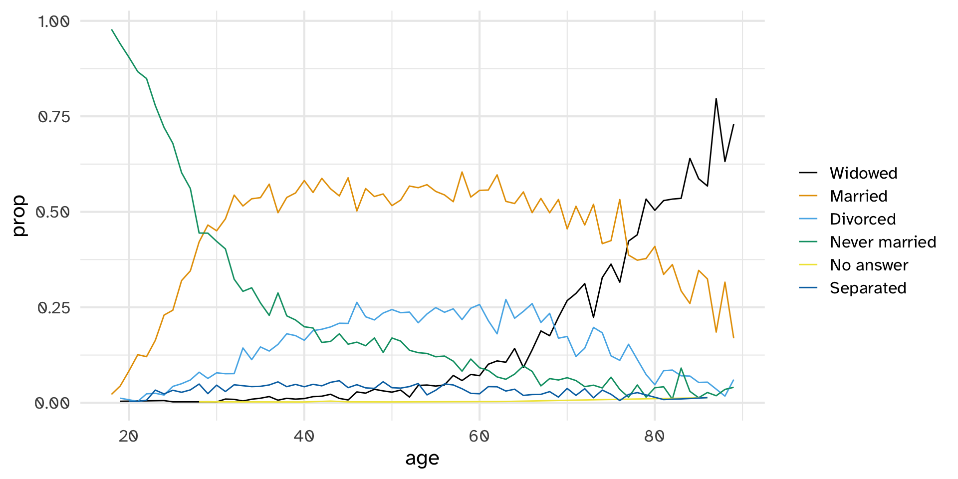
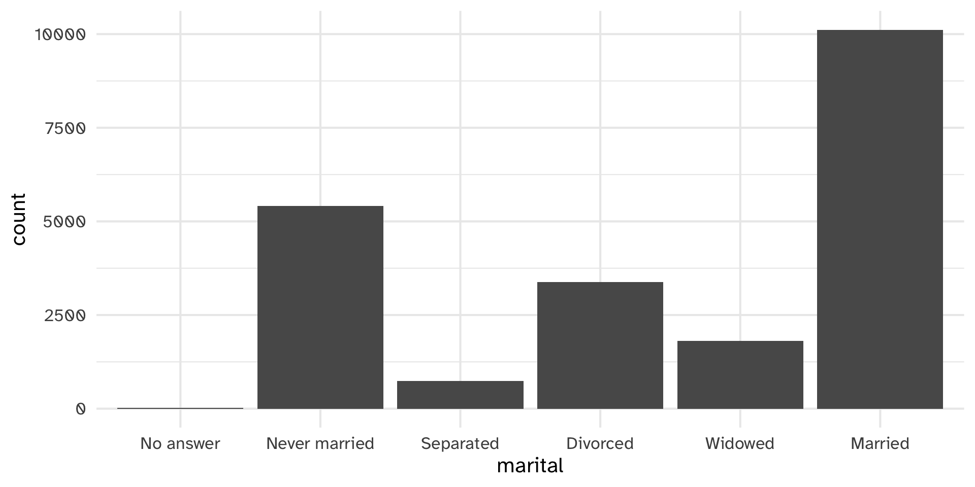
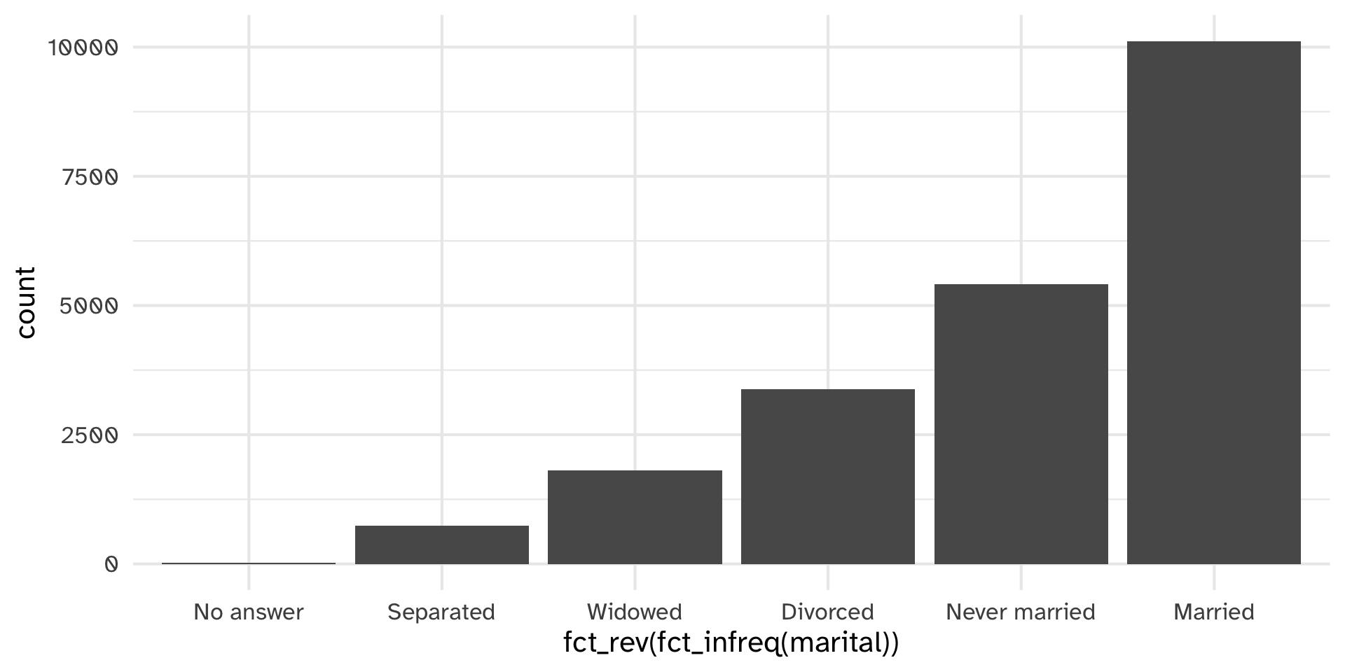
Reorder marital
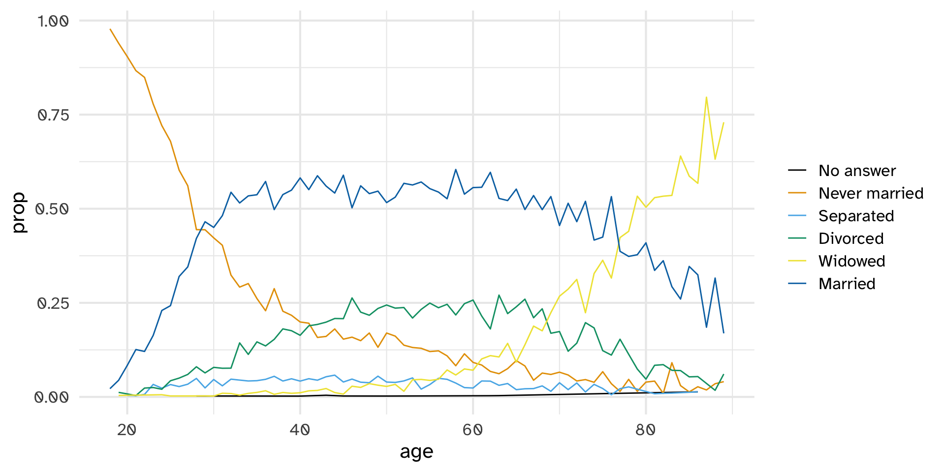
Reorder marital
Other reordering functions
Other reordering functions
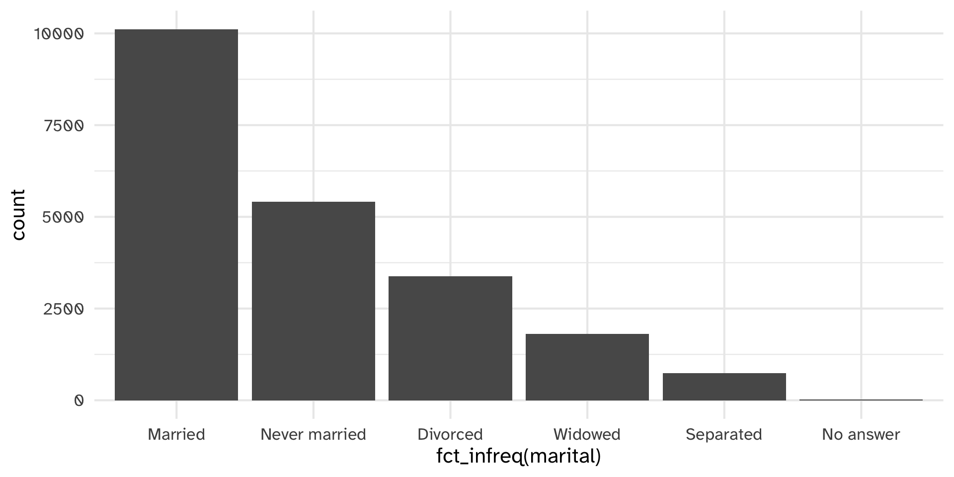
Other reordering functions
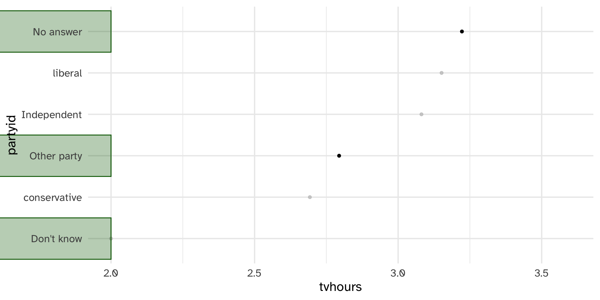
Which political leaning watches more TV?
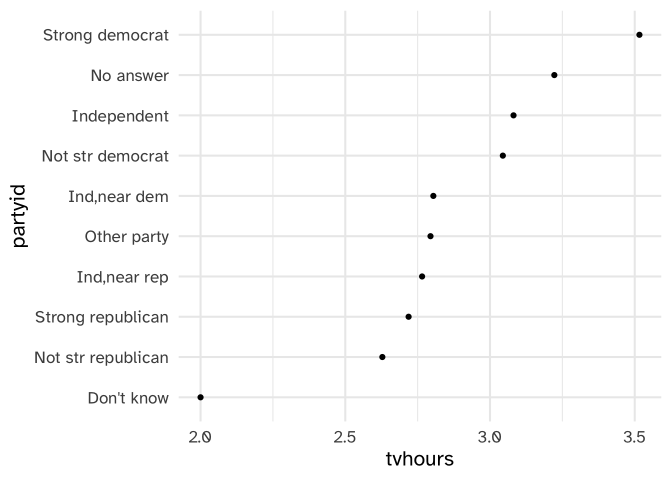
How could we improve the partyid labels?
Recoding partyid
gss_cat %>%
drop_na(tvhours) %>%
select(partyid, tvhours) %>%
mutate(partyid = fct_recode(partyid,
"Republican, strong" = "Strong republican",
"Republican, weak" = "Not str republican",
"Independent, near rep" = "Ind,near rep",
"Independent, near dem" = "Ind,near dem",
"Democrat, weak" = "Not str democrat",
"Democrat, strong" = "Strong democrat")) %>%
group_by(partyid) %>%
summarize(tvhours = mean(tvhours)) %>%
ggplot(aes(tvhours, fct_reorder(partyid, tvhours)))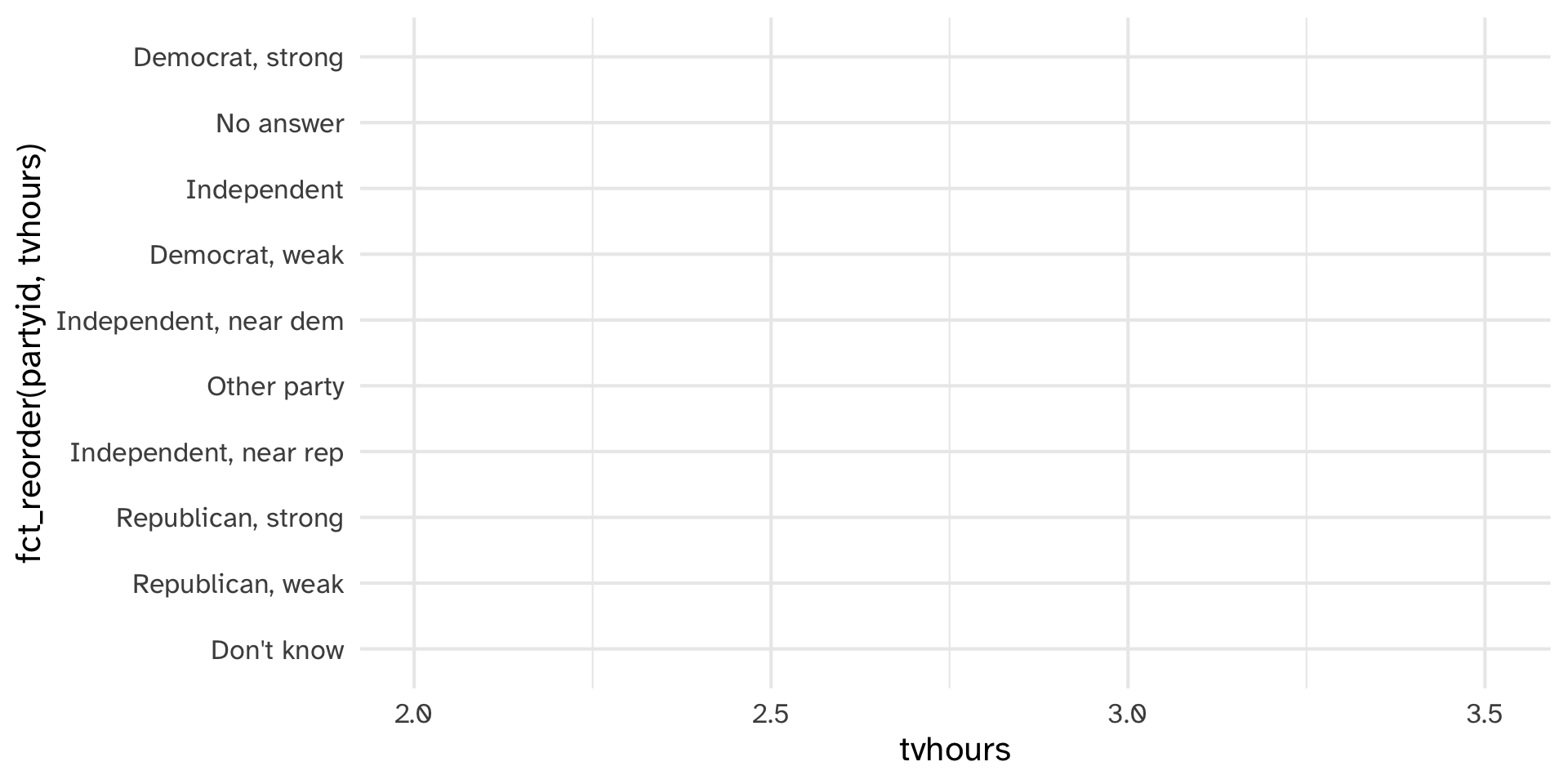
Recoding partyid
gss_cat %>%
drop_na(tvhours) %>%
select(partyid, tvhours) %>%
mutate(partyid = fct_recode(partyid,
"Republican, strong" = "Strong republican",
"Republican, weak" = "Not str republican",
"Independent, near rep" = "Ind,near rep",
"Independent, near dem" = "Ind,near dem",
"Democrat, weak" = "Not str democrat",
"Democrat, strong" = "Strong democrat")) %>%
group_by(partyid) %>%
summarize(tvhours = mean(tvhours)) %>%
ggplot(aes(tvhours, fct_reorder(partyid, tvhours))) +
geom_point()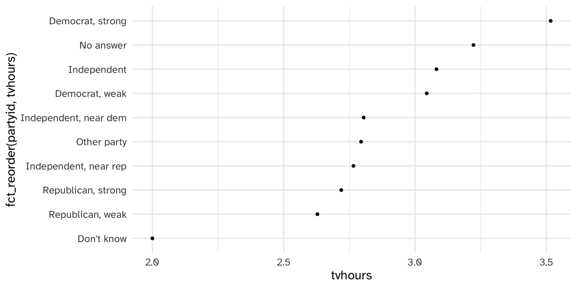
Recoding partyid
gss_cat %>%
  drop_na(tvhours) %>%
select(partyid, tvhours) %>%
mutate(partyid = fct_recode(partyid,
"Republican, strong" = "Strong republican",
"Republican, weak" = "Not str republican",
"Independent, near rep" = "Ind,near rep",
"Independent, near dem" = "Ind,near dem",
"Democrat, weak" = "Not str democrat",
"Democrat, strong" = "Strong democrat")) %>%
group_by(partyid) %>%
summarize(tvhours = mean(tvhours)) %>%
ggplot(aes(tvhours, fct_reorder(partyid, tvhours))) +
geom_point() +
labs(y = "partyid")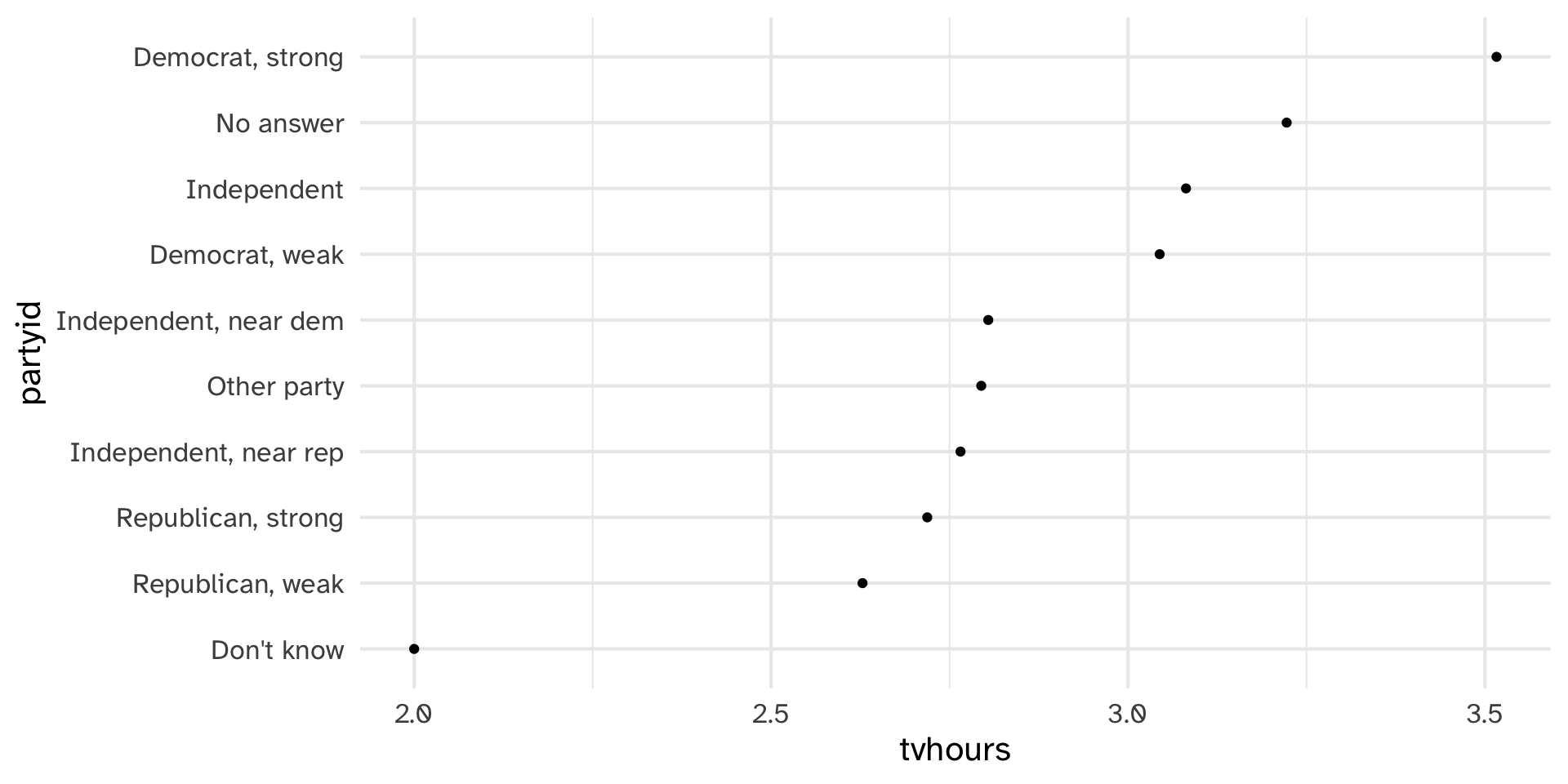
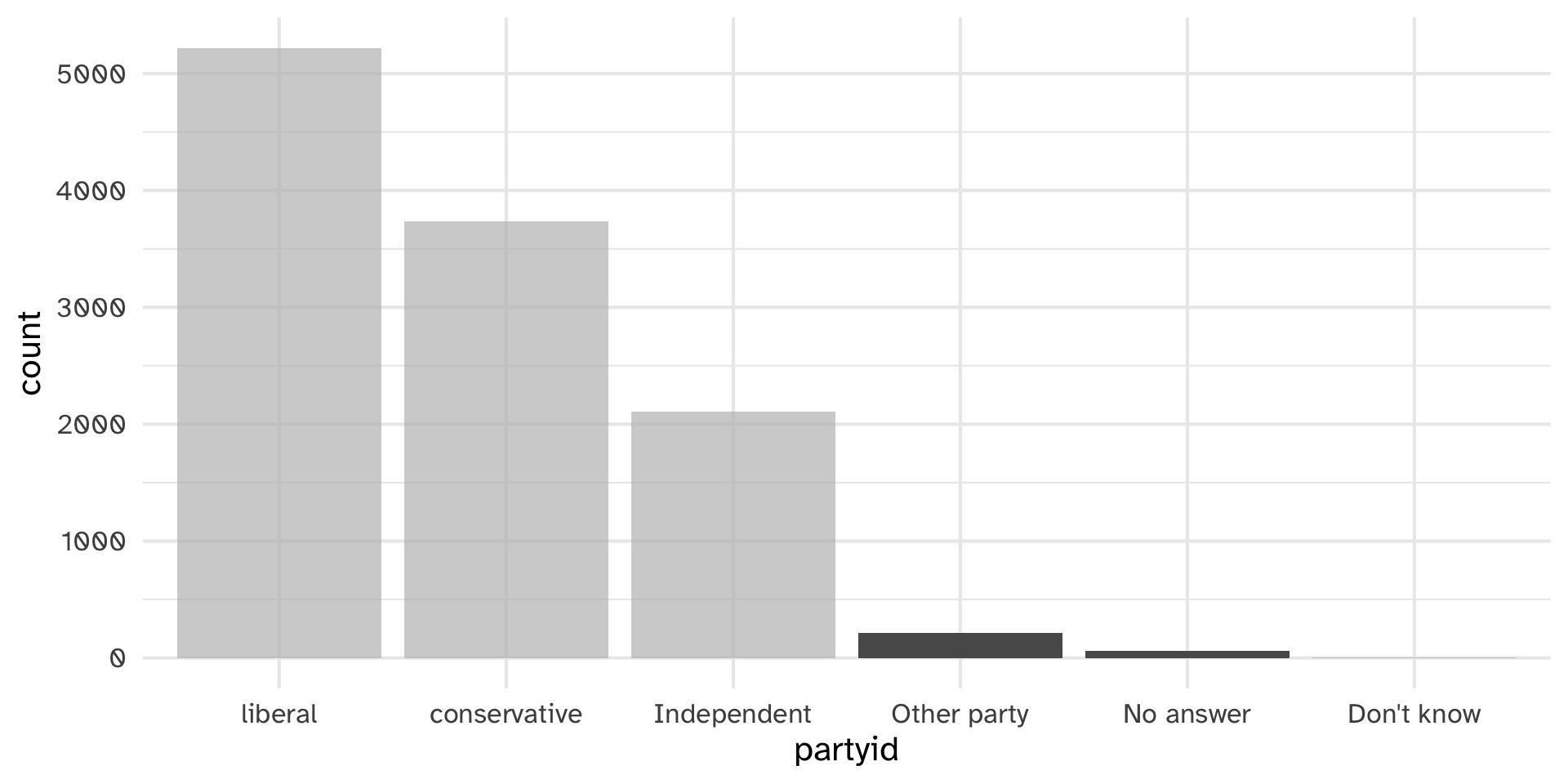
How can we combine these factor levels?
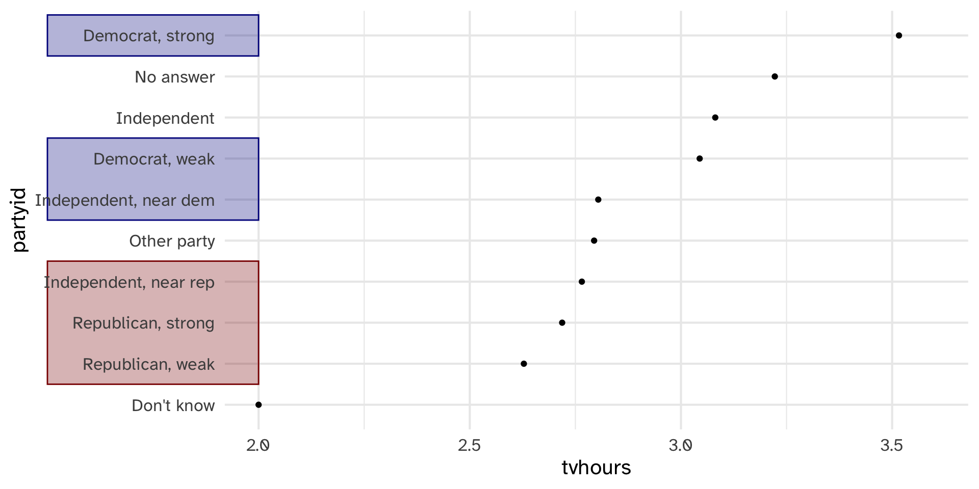
Collapsing partyid
gss_cat %>%
drop_na(tvhours) %>%
select(partyid, tvhours) %>%
mutate(
partyid =
fct_collapse(
partyid,
conservative = c("Strong republican",
"Not str republican",
"Ind,near rep"),
liberal = c("Strong democrat",
"Not str democrat",
"Ind,near dem"))
) %>%
group_by(partyid) %>%
summarize(tvhours = mean(tvhours)) %>%
ggplot(aes(tvhours, fct_reorder(partyid, tvhours)))
Collapsing partyid
gss_cat %>%
  drop_na(tvhours) %>%
select(partyid, tvhours) %>%
mutate(
partyid =
fct_collapse(
partyid,
conservative = c("Strong republican",
"Not str republican",
"Ind,near rep"),
liberal = c("Strong democrat",
"Not str democrat",
"Ind,near dem"))
) %>%
group_by(partyid) %>%
summarize(tvhours = mean(tvhours)) %>%
ggplot(aes(tvhours, fct_reorder(partyid, tvhours))) +
geom_point()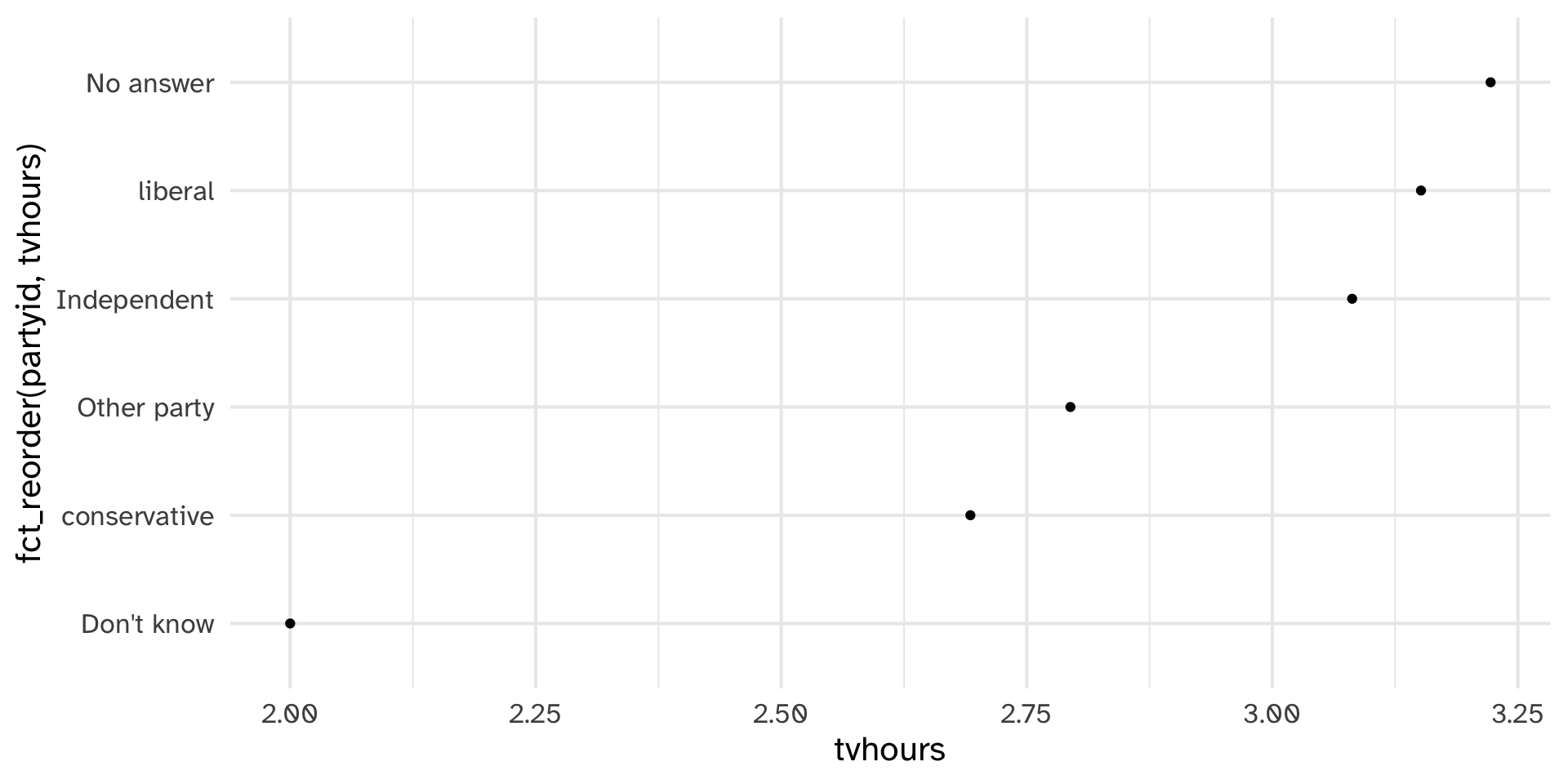
Collapsing partyid
gss_cat %>%
  drop_na(tvhours) %>%
  select(partyid, tvhours) %>%
  mutate(
    partyid =
      fct_collapse(
        partyid,
        conservative = c("Strong republican",
                         "Not str republican",
                         "Ind,near rep"),
        liberal = c("Strong democrat",
                    "Not str democrat",
                    "Ind,near dem"))
) %>%
group_by(partyid) %>%
summarize(tvhours = mean(tvhours)) %>%
ggplot(aes(tvhours, fct_reorder(partyid, tvhours))) +
geom_point() +
labs(y = "partyid")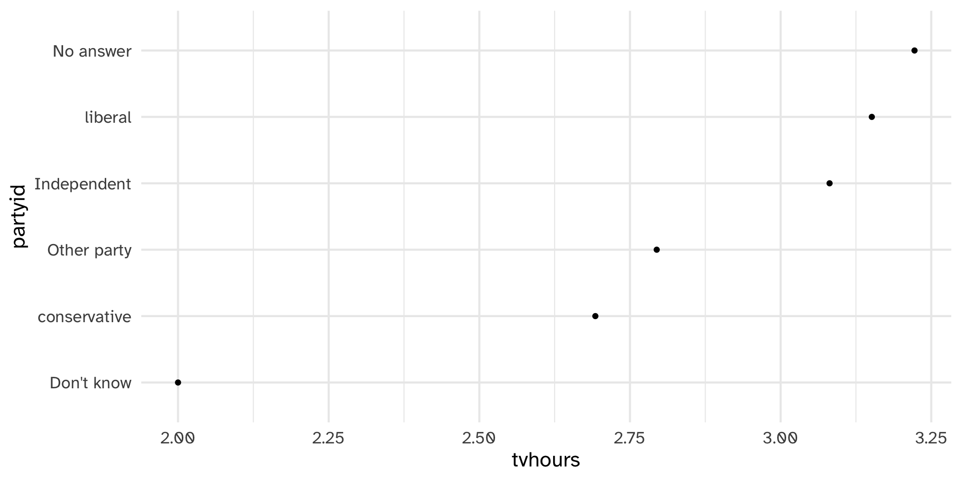
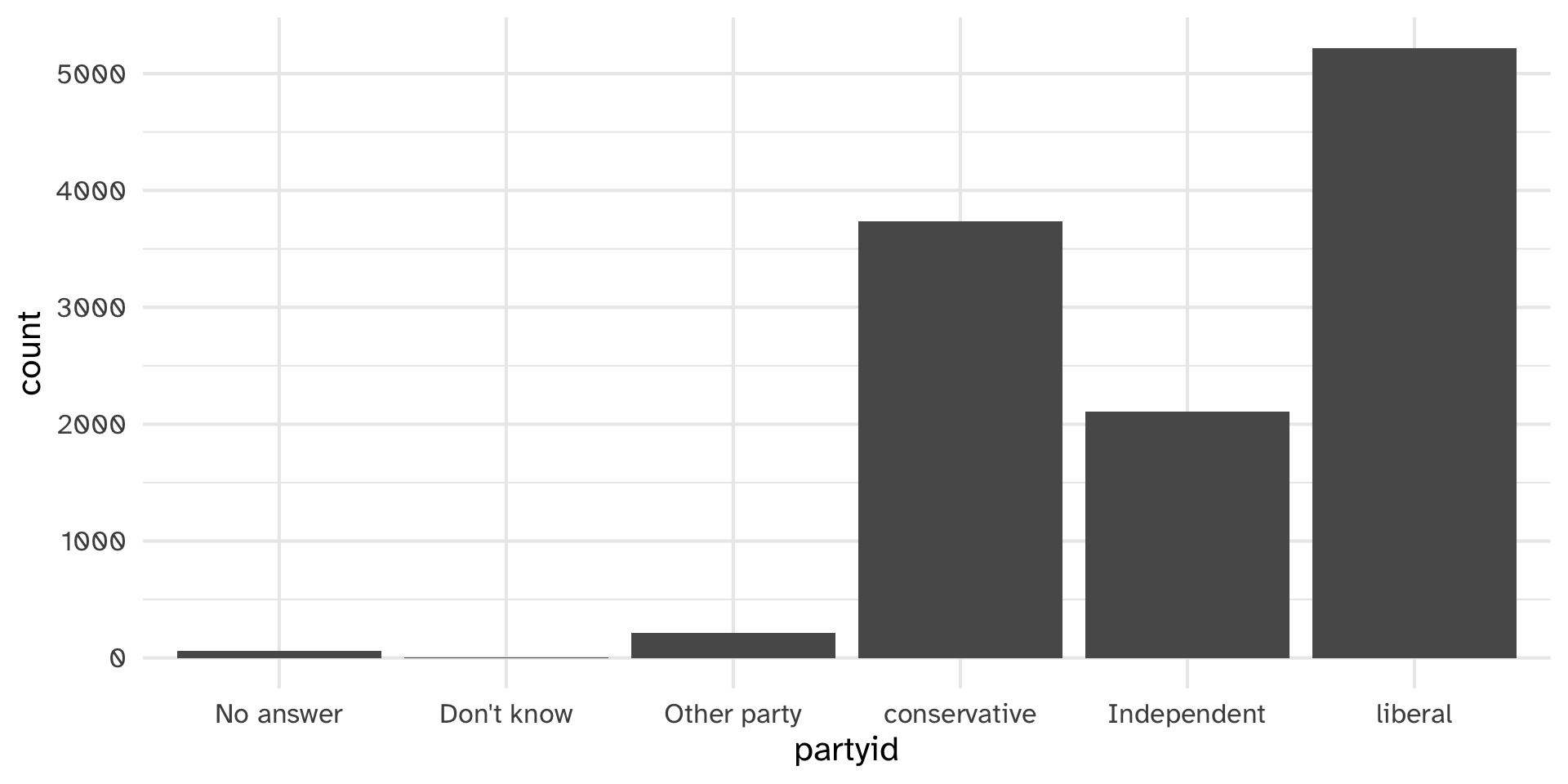
There are relatively few points in each of these groups
There are relatively few points in each of these groups
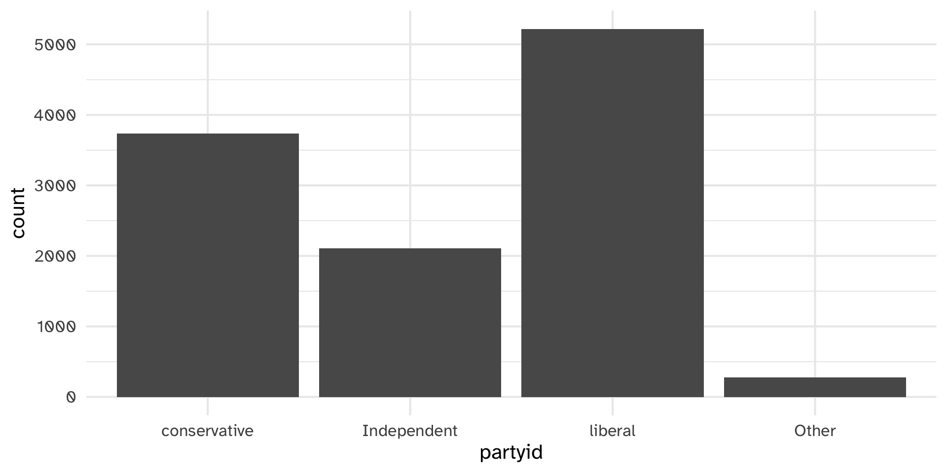
Lumping parytid
Lumping parytid
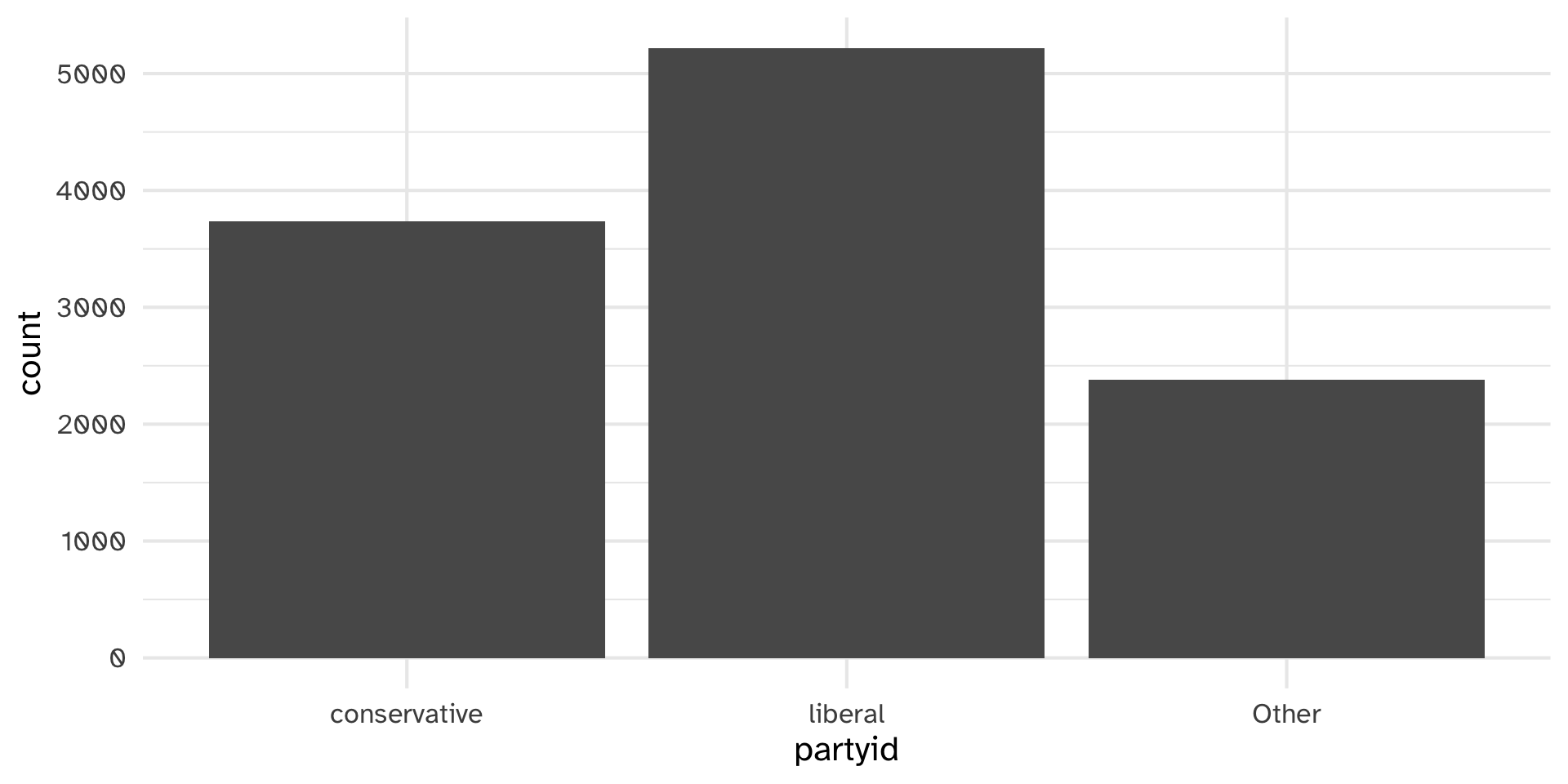
Lumping parytid
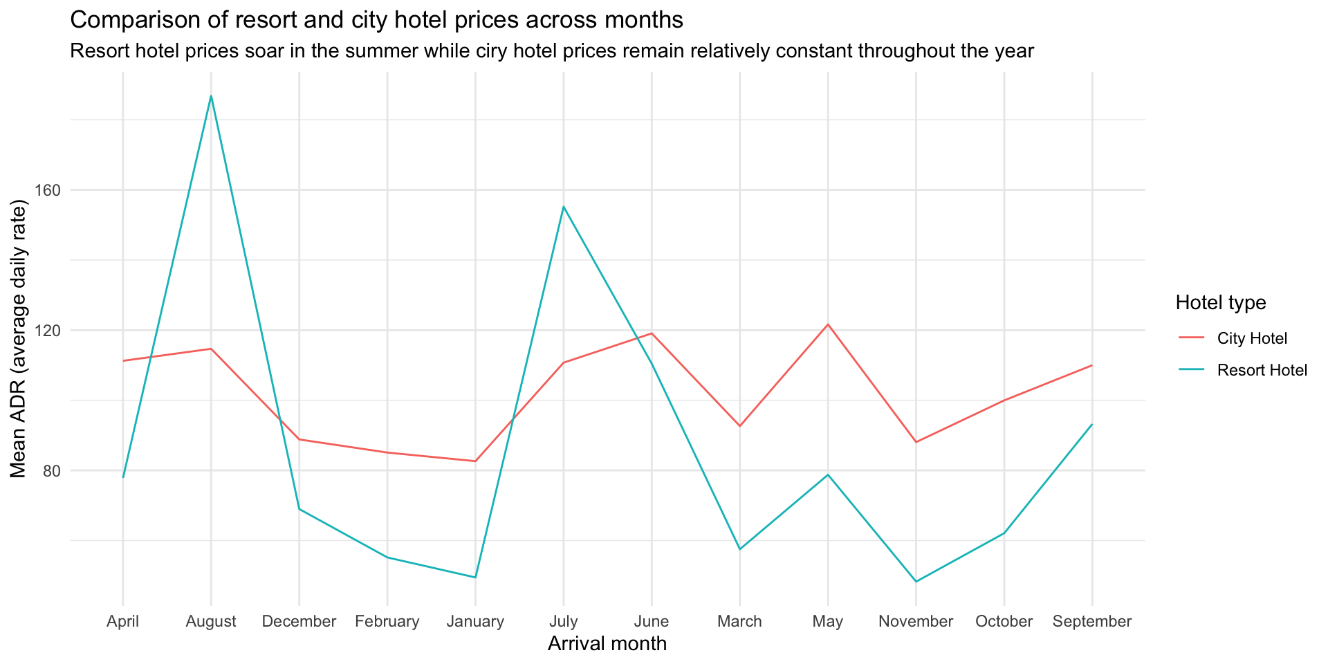
Your turn: hotel bookings
The remainder of the activity file has you fixing up some plots using hotel bookings data from Tidy Tuesday